Power Secant Method applied to natural frequency extraction
of Timoshenko beam structures
Abstract
This work deals with an improved plane frame formula-tion whose exact dynamic stiffness matrix (DSM) presents, uniquely, null determinant for the natural frequencies. In comparison with the classical DSM, the formulation herein presented has some major advantages: local mode shapes are preserved in the formulation so that, for any positive frequency, the DSM will never be ill-conditioned; in the ab-sence of poles, it is possible to employ the secant method in order to have a more computationally efficient eigenvalue extraction procedure.
Applying the procedure to the more general case of Timo-shenko beams, we introduce a new technique, named “power deflation”, that makes the secant method suitable for the transcendental nonlinear eigenvalue problems based on the improved DSM.
In order to avoid overflow occurrences that can hinder the se-cant method iterations, limiting frequencies are formulated, with scaling also applied to the eigenvalue problem. Comparisons with results available in the literature demon-strate the strength of the proposed method. Computational efficiency is compared with solutions obtained both by FEM and by the Wittrick-Williams algorithm.
Keywords
exact modal analysis, dynamic stiffness matrix, secant method, power deflation.
C.A.N. Dias∗
Group of Solid Mechanics and Structural Im-pact, Department of Mechatronics and Me-chanical System Engineering, University of S˜ao Paulo, S˜ao Paulo – 05508-900 – Brazil
Received 23 Mar 2010; In revised form 21 Jun 2010 ∗Author email: [email protected]
1 INTRODUCTION
Using an improved DSM, exact mode shape and natural frequency calculation of Euler-Bernoulli skeleton structures is discussed at length by Dias and Alves [4]. According to the Euler-Bernoulli theory, the beam transverse vibrations are only due to bending deflection. Hence, shear deflection is not taken into account, which restricts the work in [4] to the slender members and low order modes.
concomitantly the bending and shear deflections as well as the mass and the rotatory inertia per unit length.
Timoshenko beam theory will not be developed in detail here. For the purposes of the present work, we will use the theoretical results presented in Ref. [5]. A complete basic text on the theory and some of its applications can be found in Ref. [8]. Additionally, greater elucidation about the theory can be gathered from [7] and [9].
We stress that in the vibration analysis, the concept of slenderness is associated with the distance between null bending moments. Hence, even for slender beams, when the modal order increases, the shear deflection and the rotatory inertia will have an increasing influence on the natural frequencies. We may conclude, therefore, that using the Timoshenko theory is always more suitable when there are short members in the model and/or there is an interest in calculating modes of a higher order. Nevertheless, as shown, the price paid for using this theory reflects the mathematical complexity, which is greater than for the simpler Euler-Bernoulli theory.
Additionally, as the very title of Ref. [5] suggests, it can be interesting to compute the effect of axial load in flexural vibrations. When a beam suffers transverse displacement, its cross-sections suffer translations and rotations in such a manner that the axial loads perform work. If such work is added to the total amount of the elastic energy, the natural frequencies are affected. Therefore, tensile axial loads increase the natural frequencies, while, inversely, compression axial loads decrease the natural frequencies. In this last case, depending on the magnitude of the load, the “dynamic buckling” phenomenon can occur, which is characterized by the total nullification of the bending rigidity of the beam.
The fundamentals of the dynamic problem herein investigated are given in sections 2 and 3, which lead to the DSM formulation given in section 4. Section 5 investigates the numerical approach necessary for the implementation of the secant method [1]. In section 6, this method is modified to accommodate special characteristics of the non-linear transcendental eigenvalue problem explored here.
In this context, two particular numerical aspects are discussed: overflow occurrences and deflation of the DSM determinant.
Because the secant method is an iterative process, its implementation is limited by the computer numerical structure such that overflow occurrences should be predicted and circum-vented; without such planning, this process will certainly fail. Therefore, for the calculation of the hyperbolic function arguments as well as for the DSM determinant calculation, the numerical techniques described in section 5.3 should be considered.
For linear eigenvalue problems, whose similarity has been established by the finite elements method [1], the dynamic stiffness matrix determinant is a polynomial of equal or lesser order than the number of degrees of freedom. In this case, polynomial deflation [1, 13] works perfectly as an auxiliary technique of the secant method, allowing for iterative calculation of a certain eigenvalue, in a recursive process, if the lower order eigenvalues are known.
section 6 the technique called “power deflation”: in the calculation of thenth-order eigenvalue, the determinant is deflated by a product of monomial powers; each one of these containing an eigenvalue whose order is lower than n.
2 MEMBER EQUILIBRIUM EQUATIONS
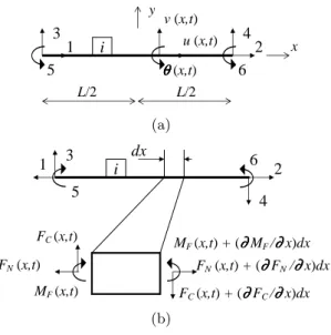
For an elementary volume of lengthdx(Fig. 1), the equilibrium of lateral forces can be written as:
FC(x, t)=m∂2v(x, t)/∂t2 (1)
whereFC(x, t) is the shear force due to bending,m=ρAis the uniform distribution mass and
v(x, t) is the transverse displacement.
Analogously, the equilibrium of the elementary volume moments gives:
FC(x, t)=∂MF(x, t)/∂x+P ∂v(x, t)/∂x−j∂2θ(x, t)/∂t2 (2)
where MF(x, t) is the bending moment, j = ρI is the uniformly distributed rotatory inertia,
θ(x, t) is the angle of rotation of the cross-section, andP is a static axial load.
The static axial load is supposedly time-invariant, constant throughout the length and positive under tensile condition.
On the other hand, the shearing condition of the elementary volume can be written as:
θ(x, t)=[1+P/(GAS)]∂v(x, t)/∂x−FC(x, t)/(GAS) (3)
whereG=E/[2(1+υ)]is the shear modulus andAS is the shear area that is given as a fraction
of the total area of the cross-section (A). The shear area characterizes the stiffness in relation to the deflection due to shear, so that ifAS =∞there is no such deflection.
Thus, eliminating FC(x, t) and MF(x, t) from these equations, it results in the following
differential equation, applicable for both transverse displacement and rotation [5]:
m∂2(
●)/∂t2−P ∂2(●)/∂x2−EI[1+P/(GAS)]∂4(●)/∂x4+
+mj/(GAS)∂4(●)/∂t4−{j[1+P/(GAS)]−mEI/(GAS)}∂4(●)/∂x2∂t2=0 (4)
where the dot denotes v(x, t) or θ(x, t). Noted in this equation is the existence of crossed terms that are involved in the relations between the beam parameters: EI =flexural rigidity, GAS =shear rigidity, m=mass per unit length, j= rotatory inertia andP =static axial load.
Additionally, using the same elementary volume of length dx (Fig. 1), the dynamic equi-librium of axial forces, from which P is excluded because it is constant, can be written as:
FN(x, t)=m∂2u(x, t)/∂t2 (5)
L/2 L/2
x 1
3
5
2 4
6 y
i
θθθθ (x,t) u (x,t) v (x,t)
(a)
2
4 6 3
1
5 i
MF (x,t) + (∂∂∂∂ MF /∂∂∂∂ x)dx
FC (x,t) + (∂∂∂∂ FC /∂∂∂∂ x)dx FN (x,t) + (∂∂∂∂ FN /∂∂∂∂ x)dx
dx
MF (x,t)
FC (x,t)
FN (x,t)
(b)
Figure 1 Timoshenko beam member at local coordinates: (a) internal & end displacements; (b) internal & end forces.
3 MEMBER EQUILIBRIUM SOLUTION
In free vibration, the displacements are synchronous and harmonic and can be written as:
u(x, t)=ϕu(x)sin(ωt) Axial Translations v(x, t)=ϕv(x)sin(ωt) Lateral Translations θ(x, t)=ϕθ(x)sin(ωt) In Plane Rotation
(6)
stressing that, for the present theory, the rotationθ(x, t) cannot be directly obtained from the derivative ofv(x, t), as it could in the Euler-Bernoulli theory.
Substitution of expressions (6) for displacements in the equations from the previous section, after some algebraic transformations, leads to:
ϕu(x)=AS¯ A(x)+BC¯ A(x)
ϕv(x)=CS¯ T(x)+DC¯ T(x)+ES¯ H(x)+F C¯ H(x) (7)
ϕθ(x)=θT[CC¯ T(x)−DS¯ T(x)]+θH[EC¯ H(x)+F S¯ H(x)]
where ¯A,B,¯ C,¯ D,¯ E¯and ¯F are integration constants to be determined by using appropriate boundary conditions,θT and θH are parameters to be given forward and:
SA(x)=sin(βAx) CA(x)=cos(βAx)
ST(x)=sin(βTx) CT(x)=cos(βTx)
SH(x)=sinh(βHx) CH(x)=cosh(βHx)
(8)
FN(x, t)=ϕN(x)sin(ω t) Normal Forces
FC(x, t)=ϕC(x)sin(ω t) Shear Forces
MF(x, t)=ϕF(x)sin(ω t) Bending Moments
(9)
with
ϕN(x)=FA[AC¯ A(x)−BS¯ A(x)]
ϕC(x)=−FT[CC¯ T(x)−DS¯ T(x)]+FH[EC¯ H(x)+F S¯ H(x)] (10)
ϕF(x)=−MT[CS¯ T(x)+DC¯ T(x)]+MH[ES¯ H(x)+F C¯ H(x)]
where the parameters FA, FT, FH, MT andMH are given forward.
For convenience, we define the following non-dimensional parameters:
Ω2(ω)=ω2/γ2 Frequency (11)
r2=I/(AL2) Rotatory Inertia (12)
s2=EI/(GASL2) Shear Deflection (13)
p2=−P L2/EI Axial Load (14)
ξ2=1−s2p2 (15)
η2=r2ξ2+s2 (16)
where, in Eq. (11) we have:
γ[rad/s]=√EI/mL4 (17)
Thus, we finally write:
θT(ω)=[ξ2α2T(ω)−s 2
Ω2(ω)]/[αT(ω)L]
θH(ω)=[ξ2α2H(ω)+s2Ω2(ω)]/[αH(ω)L]
FA(ω)=EAβA(ω)
FT(ω)=EIθT(ω)βT2(ω)−P βT(ω)−jω2θT(ω) (18)
FH(ω)=EIθH(ω)βH(2 ω)+P βH(ω)+jω2θH(ω)
MT(ω)=EIβT(ω)θT(ω)
MH(ω)=EIβH(ω)θH(ω)
where
βA(ω)=αA(ω)/L
βT(ω)=αT(ω)/L (19)
with the non-dimensional parametersαdefined by:
αA(ω)=ω √
mL2/EA=(γ/√EA/mL2)Ω(ω) (20)
αT(ω)=[∆˜(ω)+∆¯(ω)]1/2/(2ξ2)1/2 (21)
αH(ω)=[∆˜(ω)−∆¯(ω)]1/2/(2ξ2)1/2 (22)
being
˜
∆(ω)=[∆¯2(ω)+δ2(ω)]1/2 (23)
¯
∆(ω)=p2+η2Ω2(ω) (24)
δ2(ω)=4ξ2[1−r2s2Ω2(ω)]Ω2(ω) (25)
4 ASSESSMENT OF THE EXACT DYNAMIC STIFFNESS MATRIX (DSM)
4.1 Element local dynamic stiffness matrix
Employing the convention for the end displacement and the end forces shown in Fig. 1, as well as the origin there indicated for the local reference system, and defining forJ =A, T orH :
SJ−=SJ(x=−L/2); SJ+=SJ(x=+L/2)
CJ−=CJ(x=−L/2); CJ+=CJ(x=+L/2)
(26)
the dynamic stiffness matrix of an axially loaded Timoshenko member is given by:
KD(ω)=ϕϕϕP(ω)ϕϕϕ−Q1(ω) (27)
where the matricesϕϕϕQ andϕϕϕP are, respectively:
End displacements versus integration constants relationship
ϕϕϕQ(ω)= ⎡⎢ ⎢⎢ ⎢⎢ ⎢⎢ ⎢⎢ ⎢⎢ ⎢⎣
+SA− +CA− 0 0 0 0
+SA+ +CA+ 0 0 0 0
0 0 +S−T +CT− +SH− +CH−
0 0 +S+T +CT+ +SH+ +CH+
0 0 +θTCT− −θTST− +θHCH− +θHSH−
0 0 +θTCT+ −θTST+ +θHCH+ +θHSH+ ⎤⎥ ⎥⎥ ⎥⎥ ⎥⎥ ⎥⎥ ⎥⎥ ⎥⎦
End forces versus integration constants relationship
ϕ ϕ ϕP(ω)=
⎡⎢ ⎢⎢ ⎢⎢ ⎢⎢ ⎢⎢ ⎢⎢ ⎢⎣
+FACA− −FASA− 0 0 0 0
+FACA+ −FASA+ 0 0 0 0
0 0 −FTCT− +FTST− +FHCH− +FHSH−
0 0 −FTCT+ +FTST+ +FHCH+ +FHSH+
0 0 −MTS−T −MTCT− +MHSH− +MHCH−
0 0 −MTS+T −MTCT+ +MHSH+ +MHCH+ ⎤⎥ ⎥⎥ ⎥⎥ ⎥⎥ ⎥⎥ ⎥⎥ ⎥⎦
(29)
In the expressions (28) and (29), the parametersθT,θH,FA,FT,FH,MT andMH depend
on the frequency ω and are defined by Eqs. (18).
By the usual FEM procedures, the matrix of expression (27), after applied to each member of the model, is useful to assemble the classical global DSM [5]. However, for frequencies that coincide with the natural frequencies of the members in the clamped-clamped condition, the classical DSM has poles, not roots.
This can be easily seen by observing that the matrix φQ(ω) has no inverse when ω is one of the natural frequencies of the member in the clamped-clamped condition so that, as consequence, the DSM determinant grows to infinity.
For this reason, the classical DSM is not suitable in an iterative method that needs deter-minant values to estimate the natural frequencies. To overcome this difficulty, in the following section it is shown how the matrices φP(ω) and φQ(ω) can be used in order to assemble an
improved version of the global DSM that has no poles [4]. Then, the improved DSM can be used to extract eigenvalues by the secant method [1], as it will be presented in section 6.
4.2 Improved global dynamic stiffness matrix
By applying the standard FEM procedures, the process by which the matrices ϕϕϕP(ω) and
ϕϕϕQ(ω) are employed for the in-plane model assembly, in the light of the Timoshenko theory,
follows the same steps that are described in Ref. [4] for the Euler-Bernoulli theory. For the sake of brevity, the details will not be presented here. The terms are:
M Total number of members of the model; N Total number of nodal degrees of freedom;
Qo Vector of the amplitudes of the nodal displacements;
Θ Vector that contains the constants of integration of all the members; ˆ
Ω Matrix that unites the nodal concentrated masses and springs;
ψQ Matrix that determines the connection between the members of the model; ΦP Matrix that unites the matricesϕϕϕP(ω) of all the members;
ΦQ Matrix that unites the matricesϕϕϕQ(ω) of all the members.
⎡⎢ ⎢⎢ ⎢⎢ ⎢⎣
ΦQ(ω) 6M−by−6M
−ψQ 6M−by−N ψTQΦP(ω)
N−by−6M
ˆ Ω(ω)
N−by−N ⎤⎥ ⎥⎥ ⎥⎥ ⎥⎦ ´¹¹¹¹¹¹¹¹¹¹¹¹¹¹¹¹¹¹¹¹¹¹¹¹¹¹¹¹¹¹¹¹¹¹¹¹¹¹¹¹¹¹¹¹¹¹¹¹¹¹¹¹¹¹¹¹¹¹¹¹¹¹¹¹¹¹¹¹¹¹¹¹¹¹¹¹¹¹¹¹¸¹¹¹¹¹¹¹¹¹¹¹¹¹¹¹¹¹¹¹¹¹¹¹¹¹¹¹¹¹¹¹¹¹¹¹¹¹¹¹¹¹¹¹¹¹¹¹¹¹¹¹¹¹¹¹¹¹¹¹¹¹¹¹¹¹¹¹¹¹¹¹¹¹¹¹¹¹¹¹¹
=Ψ(ω)
⎧⎪⎪⎪ ⎨⎪⎪⎪ ⎩
Θ
6M−by−1 Qo N x1
⎫⎪⎪⎪ ⎬⎪⎪⎪ ⎭ ´¹¹¹¹¹¹¹¹¹¹¹¹¹¹¹¹¹¹¹¹¹¹¹¹¹¹¹¹¹¹¹¸¹¹¹¹¹¹¹¹¹¹¹¹¹¹¹¹¹¹¹¹¹¹¹¹¹¹¹¹¹¹
(6M+N)−by−1
= 0
(6M+N)−by−1 (30)
being necessary to search forω such that:
det{ Ψ(ω)
(6M+N)−by−(6M+N)}
=0 (31)
For this eigenvalue problem, which does not show poles in the natural frequencies [4], it is possible to obtain the roots of Eq. (31) and then return to Eq. (30) to obtain the corresponding vectors Θand Qo. The first of these vectors contains the integration constants, which in the latter instance determine the amplitudes of the internal displacements, and the second vector determines the amplitudes of the nodal displacements.
In these terms, for the calculation of each natural mode shape, the solution of Eq. (30) is based in a method that linearizes the eigenvalue problem in the vicinity of the corresponding natural frequency, as described in Ref. [4]. For the sake of brevity, this method will not be reproduced here.
In Ref. [4], a simple method of determinant tracing was presented to solve Eq. (31). Although robust, it is not computationally efficient because the method requires successive evaluations of the determinant, at frequency intervals not greater than the tolerance specified for the natural frequencies calculations. Thus, the objective is to implement the secant method with the use of power deflation, which is computationally much more efficient. Having in mind this implementation, in the following section some particular issues about the present eigenvalue problem are discussed.
Based on transcendental member stiffness matrices, Ref. [9] defines a new dynamic stiffness matrix, called K∞, which also eliminates the poles from the eigenvalue problem. However, this method requires further developments in order to include rigid off-set and end release in its formulation as well as has no direct capability to determine the local mode shapes for which
Qo =0 and Θ≠0.
5 PARTICULAR ISSUES
As we have shown, derivation of the Timoshenko theory is much more laborious than the Euler-Bernoulli theory; consequently, new physical and mathematical questions arise, which we will discuss in the following sections.
5.1 Limiting compression axial load
By imposing that the denominator in expressions (21) and (22), for the parameters αT and
ξ2=1−s2p2>0 (32)
which limits the axial load to:
∣P∣<GAS (33)
Thus, the lower the shear rigidity, GAS, the lower the axial load that can be applied.
In practical terms, for actual materials such a limit is sufficiently high to make feasible the calculation for any realistic structure.
On the other hand, even for infinite shear rigidity, the compressive axial load can be physically limited by the buckling phenomenon. As an illustrative example, we may consider the case of a simply supported beam with no shear deflection (AS = ∞ ⇒ s = 0). For this
situation of a Rayleigh beam, the equations in section 3 are applied in the appendix A and give for the natural frequencies:
fi[Hz]=iπ√i2
+P/PCR √
EI/mL4/√1
+r2(iπ)2/2 (34)
where, in accordance with the Euler buckling load : PCR=π2EI/L2 .
Hence, if the load is compressive (P < 0) and has magnitude greater or equal to the buckling load, null or complex natural frequencies will occur; a fact that characterizes the physical impossibility of dynamic equilibrium.
5.2 Transition frequency
The parameterαT, present in the arguments of the trigonometric functions, will always result
in a real number because the conditions ∂2<0 and ¯∆<0 cannot occur concomitantly.
On the other hand, the parameter αH, in the arguments of the hyperbolic functions, can
result in a real number or a purely imaginary number, without thereby implying any impossi-bility, either mathematical or physical.
In these terms, a particular frequency value exists for which the transition of αH occurs
from a real number to an imaginary number. Thus, the use of expression (25) and the condition (32) imposes that:
δ2(ω)=4ξ2[1−r2s2Ω2(ω)]Ω2(ω)=0 (35)
to obtain, from Eq. (11), the following expression for the transition frequency:
fT[Hz]= 1 2π rs
√
EI mL4 =
√
GAAS
mI /2π (36)
As noted in Eq. (36), if the shear deflection is neglected (s=0) there is no transition and overflow can occur because the hyperbolic function arguments are always real numbers. The same fact occurs when the rotatory inertia is neglected (r=0). On the other hand, it can be noted that the transition frequency does not depend on the member length and therefore it is not affected by mesh refinement.
5.3 Treatment of overflow conditions
For computer calculation, there is always an upper limit for the largest number that can be stored in the RAM (Rmax). If during some step of an iterative calculation such a limit is
surpassed, this calculation is certainly compromised due to overflow.
The equations in sections 3 and 4 have parameters that increase with the frequency ωsuch that this may lead to overflow error, particularly because hyperbolic functions are used.
Hence, to overcome overflow occurrences, appendix B is dedicated to the establishment of five possible limiting values (ΩlimJ for J = 1,2,3,4,5) for the non-dimensional frequency
Ω defined by Eq. (11). Accordingly, each member of the model will have its own limiting frequency given by:
flim[Hz]=(1/2π)min{ΩlimJ} √
EI
mL4 (37)
For a framed structure, the overall limiting frequency is the smallest value given by Eq. (37) applied for all the members. If this overall frequency is less than the maximum desired frequency, the only remaining alternative is to promote mesh refinement. As inferred from the example in Fig. 2, the shorter the elements the greater the overall limiting frequency.
On the other hand, the more refined the mesh the greater the possibility of overflow oc-currence in the calculation of the DSM determinant because the matrix order will be greater. Fortunately, as shown afterwards, scaling operation in the DSM can be employed to avoid such an occurrence.
In order to obtain a more elucidative visual effect, the example in Fig. 2 uses an intention-ally low Rmax value. In Fig. 2a, it can be observed how each of the non-dimensional limiting
frequencies ΩlimJ varies with the mesh refinement. By applying Eq. (37), Fig. 2b shows the
behavior of the overall limiting frequency flim. Finally, Fig. 2c shows how mesh refinement
increases the modal order of the greatest natural frequency that can be calculated.
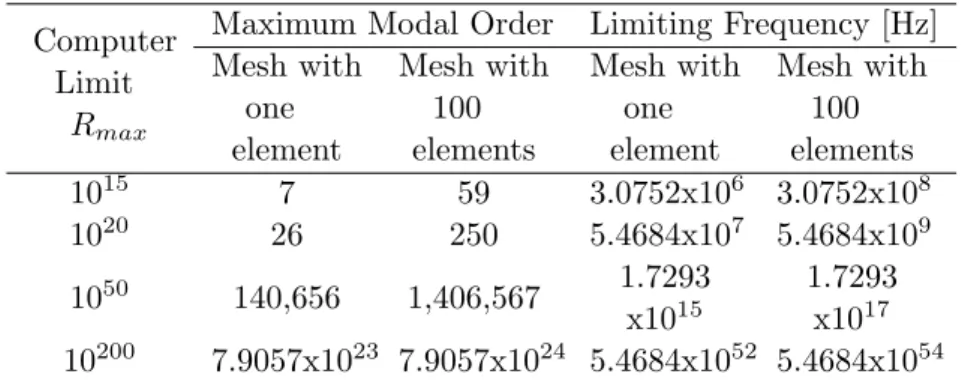
Table 1 explores how the increase in the order of Rmax, up to a compatible value with
the real computer capacity, affects the modal order of the greatest natural frequency that can be calculated. In general, it is assumed that only unrealistic data should cause relevant computational limitation by overflow error. For example, from the situation in the last line in Table 1, if an unrealistic axial load P = +10100ton is applied, the maximal calculable mode
(a)
(b)
(c)
Figure 2 Overflow limits for a simply supported beam: (a) non-dimensional limiting frequenciesΩlimJ; (b)
overall limiting frequencyflim [Hz]; (c) maximum modal orderRmax=1015;E=2000 ton/cm 2
; υ=0.3;ρ=8x10⁻⁹ton.s2/cm4;P= +15.0 ton;L=100 cm;A=10.0 cm2;AS=(5/6)A.
Table 1 Maximum obtainable modal order for the example of Fig.2.
Computer Limit
Rmax
Maximum Modal Order Limiting Frequency [Hz] Mesh with
one element
Mesh with 100 elements
Mesh with one element
Mesh with 100 elements
1015 7 59 3.0752x10⁶ 3.0752x10⁸
1020 26 250 5.4684x10⁷ 5.4684x10⁹
1050 140,656 1,406,567 1.7293
x1015
1.7293 x10¹⁷
Dynamic stiffness scaling
We consider the dynamic stiffness matrix, which is defined in Eq. (30), now affected by a real and positive scaling constantαG:
˜
Ψ(ω)=αGΨ(ω) (38)
so that the calculation of the DSM determinant can be written as:
det[Ψ˜(ω)]=αG6M+Ndet[Ψ(ω)] (39)
whereM and N are positive integers, which represent, respectively, the number of elements of the model and the total number of nodal degrees of freedom.
Thus, we note from Eq. (39) that the scaling constant αG can be used to change the
magnitude of the determinant result without, in essence, affecting the eigenvalue problem. With no changes in the mode shapes and natural frequency results, a scaling constantαG
lower than the unit can avoid the overflow occurrence.
To predict a suitable value of αG, we apply a process of trial and error, in the following
terms:
1. The overflow condition is tested for a value less than Rmax, through the appropriate
adoption of the safety coefficientSF >1: Vmax=10[log(Rmax)/SF].
2. In the calculation of the first natural frequency, while the determinant is greater than Vmax, theαG value is diminished and the iterative process is restarted.
3. Once a natural frequency is obtained, the maximum current determinant value (Dmax),
if greater than Vmax, is used to diminish the current scaling constant by using: αG =
αG[Dmax/Vmax]1/(6M+N).
For some methods other than the secant method, like bisection, scaling of the dynamic stiffness determinant could be conveniently performed during calculation by maintaining its magnitude within an allowable range and storing an additional integer exponent, so avoiding the need of predicting a suitable value for αG.
6 POWER SECANT METHOD
The objective here is to elaborate a method that serves as an alternative to the tracing method of Ref. [4], leading to a search for the natural frequencies that are computationally more efficient.
We begin with the discussion of the simple secant method; afterwards, we address the question of polynomial deflation, and, finally, we deal with power deflation.
need deflation. If, on the other hand, the function has more than one root, the method can still work under the following conditions:
• If the starting points are chosen below the first root, convergence to this root will occur;
• If the starting points are sufficiently close to a given root, convergence to this root will occur.
In the case of functions with several roots, we can apply the deflation technique to extract them in ascending order [1, 13]. Thus, by removing the first root by deflation, if the starting points are chosen from below the second root, convergence to this second root will occur. In succession: being known the (n-1) lower roots, if by deflation these roots are removed, when choosing starting points from below thenth root, convergence to this root will occur.
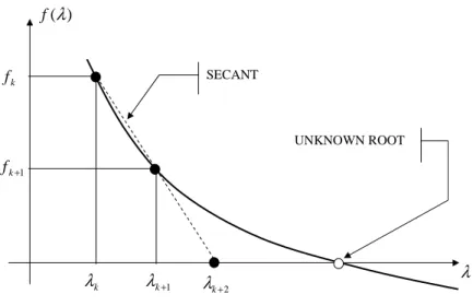
6.1 Simple Secant Method
Observing the secant method in its simplest form in Fig. 3, we can develop through recursive application of the equation that represents the intersection of the secant line with theλ axis:
λk+2=λk+1−fk+1(λk+1−λk)/(fk+1−fk) (40)
Beginning with k = 1, so that it is necessary to arbitrate two starting pointsλ1 and λ2, the
iterations are interrupted when a tolerance test is met, as prescribed by:
∣λk+2−λk+1∣≤10−dλk+2 (41)
wheredis the number of significant digits that are desired for the approximation to the sought root. If during the iterations fk = fk+1occurs, the method fails in an unrecoverable way. In
general, the method should not be directly applied in case the function has null derivative points, as when more than one root exists. In this context, the deflation technique becomes relevant.
6.2 Polynomial deflation
Lets suppose that the functionf(λ), from which we desire to extract the roots, is a polynomial of order N, with N real and distinct roots. Thus, the function is known in an explicit form from its coefficients an:
f(λ)=
N
∑
n=0
anλn (42)
or the function can be imagined in the implicit factorized form, described by monomial products involving its roots ¯λn:
f(λ)=(λ−λ¯1)(λ−¯λ2)...(λ−λ¯N)= N
∏
n=1
2
+ k
λ
k
λ λk+1
λ
) (λ
f
1
+ k f
k f
UNKNOWN ROOT SECANT
Figure 3 Simple secant method.
As shown before, the simple secant method can be applied for calculation of the first root if the starting points that are lower than this root. Once the first root ¯λ1 is obtained, a new
function is found by using the following deflation:
F2(λ)=f(λ)/(λ−λ¯1) (44)
Now, the first root of the deflated polynomial F2(λ)is in the position of the second root
of the original polynomialf(λ). Thus, the secant method can be now applied on the deflated polynomial. If the starting points are chosen below this first root, the method converges to the second root.
Such a deflation procedure can be generalized for the progressive calculation of all the roots.
Fn(λ)=f(λ)/[(λ−λ¯1)(λ−λ¯2)....(λ−λ¯n−1)]=f(λ)/ n−1
∏
j=1
(λ−λ¯j) (45)
where Fn(λ) is the deflated form of the original polynomial that makes the secant method to
converge to then-order root, being necessary that all the lower (n-1) roots have already been calculated.
For the purpose of the eigenvalue extraction of a linear problem, and for the conditions that have been established here, the secant method with polynomial deflation can be applied with success even for the case of repeated natural frequencies [13].
6.3 Power deflation
arise from FEM models, the secant method can be employed without reservations. Being K
the stiffness matrix and M the mass matrix of a FEM model withN degrees of freedom:
f(λ)=det[ K ® N xN
−λ M¯ N xN
] (46)
is a polynomial of order N with a maximum of N real and non negative roots [1]. The fact that the polynomial in Eq. (46) is not known in an explicit form, like in Eq. (42), does not hinder the application of the secant method because it is still possible to make numerical evaluations of f(λ). Especially for case of Eq. (46), such numerical evaluations are more efficiently conducted through the Gauss factorization [1]:
K−λM =L(λ)D(λ)LT(λ) (47)
where L(λ) is a lower triangular matrix and D(λ) is a diagonal matrix. Once performing factorization, the determinant is simply calculated from the products of the diagonal terms of the matrix D(λ):
f(λ)=det(K−λM)= N
∏
i=1
dii(λ) (48)
On the other hand, for the improved dynamic stiffness matrix Ψin Eq. (30), the function f(λ) = det{Ψ(λ)} is not a polynomial, although it has non-negative real roots. Thus, the polynomial deflation has little or no possibility of working.
In these terms, alternatively we use the following modified version of Eq. (45), which characterizes what we call power deflation:
Fn(λ)=f(λ)/⎡⎢⎢⎢ ⎣λ
No
n−1
∏
j=1
(λ−λ¯j)Nj⎤⎥⎥⎥
⎦ (49)
where each Nj power should be determined in a manner that, given two starting points λ1n
and λ2n, the following condition is met:
[Fj(λ1n)
λ1n−λ¯j] Nj
=ζ[Fj(λ2n) λ2n−λ¯j ]
Nj
with ζ>1 (50)
For calculation of the first eigenvalue (n=1⇒j =0), we have F0(λ) =f(λ) and ¯λo =0.
Consequently, before starting the iterations for each root, it is guaranteed that the first secant line favorably intersects the λaxis at a point located ahead the starting points. Then, from Eq. (50), we can obtain the following general expression for calculating the Nj powers that
are applied in Eq. (49):
Nj ={log[(Fj(λ1n)/Fj(λ2n)]−logζ} / {log[
λ1n−λ¯j
λ2n−λ¯j]}
If this expression results in Nj <1,Nj =1 is adopted because the corresponding deflation
is not needed.
For the iterations of the first mode (n=1 ⇒j =0), we calculate N0 using Eq. (51) and
apply Eq. (49) in order to obtain F1 to use in the secant method. For the iterations of the
second mode (n = 2 ⇒ j = 1), using F1 , we calculate N1 by Eq. (51) and apply Eq. (49)
in order to obtain F2 to use in the secant method; and thus, the other following modes are
progressively calculated.
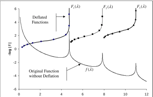
To illustrate the operation of the secant method with power deflation, or here simply called “the power secant method”, we present in Fig. 4 the results for a simple clamped-clamped Euler-Bernoulli beam. In this case, we usedζ=2 and appropriate starting points in order that convergence occurs for up to ten iterations. In the figure, we can visualize how the deflated functions converge for the eigenvalues of the problem, which are localized at the peaks of the function−log{∣f(λ)∣}.
-6 -4 -2 0 2 4 6
0 2 4 6 8 10 12
-l
o
g
|
f
|
Original Function without Deflation
Deflated Functions
) (λ
f
) (
2 λ
F F3(λ)
) (
1 λ
F
Figure 4 Application example of the power secant method (ζ=2): calculation of the first three roots of the
frequency equationf(λ)=cos(λ).cosh(λ)−1, for a clamped-clamped single Euler-Bernoulli beam.
The marks on the curves show the performed iterations.
Obviously, the success of the method, in terms of the number of iterations that are needed to achieve convergence, strongly depends on the starting points and on the appropriate choice of the parameter ζ.
Depending on the problem, the parameter ζ can be previously admitted as a constant or varied, by trial and error, until the iterative process demonstrates appropriate convergence. In this last case, in the beginning of the iterations for each root, ζ should be re-estimated whenever necessary.
Without the benefit of prior knowledge of the roots, the solution for each one of these equations uses arbitrary starting points as well as automatically determined value for the parameterζ.
We note in Table 2 that, under this more general situation useful for computer program-ming, there is a reasonable increase in the number of iterations. We also observe that the final results precisely coincide with the known solutions of the problems [2].
In spite of the number of iterations, the power secant method is always faster than the bisection method. For comparison, lets take the example of the clamped-clamped beam in Table 2. The power secant method performed 168 evaluations of the frequency equation while a bisection method needs more than 1000 evaluations to reach the same accuracy.
Table 2 Power secant method applied to single Euler-Bernoulli beams.
BCa Frequency
Equation
Mode Iter.s
Number
Power Deflation Starting Pointsb Rootc
j ζ Nj−1 λ1 λ2 λ¯j
P-P
S-S sin(λ)
1 43 16 3.00000 0.0001 0.0002 3.14159
2 48 16 2.99993 3.14164 3.14169 6.28319
3 50 16 2.99989 6.28324 6.28329 9.42478
S-P cos(λ)
1 39 8 2.00000 0.0001 0.0002 1.57080
2 48 16 2.99991 1.57085 1.57090 4.71239
3 50 16 2.99991 4.71244 4.71249 7.85398
C-C
F-F 1−cos(λ).cosh(λ)
1 74 32 8,33296 0.0002 0.0003 4.73004
2 47 16 2.99994 4.73009 4.73014 7.85320
3 47 16 2.99992 7.85325 7.85330 10.9956
F-S
C-S tan(λ)+tanh(λ)
1 44 16 3.00000 0.0001 0.0002 2.36502
2 54 16 2.99983 2.36507 2.36512 5.49780
3 57 16 2.99981 5.49785 5.49790 8.63938
F-P
C-P tan(λ)−tanh(λ)
1 47 32 5.00000 0.0001 0.0002 3.92660
2 47 16 2.99998 3,92665 3.92670 7.06858
3 55 16 2.99995 7.06863 7.06868 10.2102
C-F 1+cos(λ).cosh(λ)
1 38 8 2.00000 0.0001 0.0002 1,87510
2 43 16 2.99997 1.87515 1.87520 4.69409
3 45 16 2.99996 4.69414 4.69419 7.85476
a
Boundary condition convention: P=Pinned; C=Clamped; F=Free; S=Sliding. b
Forj>=2 both starting points must be greater than the previous root
c
Roots obtained with six digits of tolerance
7 COMPARISON EXAMPLES
The power secant method was implemented in the VIGENE program [3], which was developed on the MATLAB platform. This program is a part of the VIANDI computational system that is available for download at http://www.gmsie.usp.br .
Finally, in order to explore the entire VIGENE capability, section 7.4 presents a more complex model.
7.1 Simply supported Euler-Bernoulli beam under axial load
As shown in the appendix A, if shear deflection and rotatory inertia are disregarded, the simply supported beam has exact analytical solution, which does not require application of any iterative numerical processes. We can observe in Table 3 the perfect concordance between this analytical solution and the numerical solution of the VIGENE program.
Table 3 Natural frequencies [Hz] for a simply supported Euler-Bernoulli beam under axial load: L=10 cm; E=104ton/cm2;ρ=1 ton.s2
/cm4 ;A=π2
cm2
;I=4 cm4 Axial
Load P/PCR = 0.0 P/PCR = -0.5 P/PCR = +2.0
Mode Analyticala VIGENE Analyticala VIGENE Analyticala VIGENE
1 1.0000 1.0000 0.7071 0.7071 1.7321 1.7321
2 4.0000 4.0000 3.7417 3.7417 4.8990 4.8990
3 9.0000 9.0000 8.7464 8.7464 9.9499 9.9499
4 16.000 16.000 15.748 15.748 16.971 16.971
5 25.000 25.000 24.749 24.749 25.981 25.981
a
Analytical solution: fi[Hz]=i√i2+P/PCR
7.2 Single Timoshenko beam for various boundary conditions
For comparison, from [7] and [12] we took the examples shown in Tables 4 and 5, respectively. A good concordance can be observed between VIGENE and ANSYS programs.
Table 4 Natural frequencies [Hz] for the single Timoshenko beam of Majkut [7]: L=1 m; E =210 Gpa;
v=0.2963;ρ=7860 Kg/m3;A=0.0016 m2;AS=(5/6)A I=8.53333e−7 m4.
Case Pinned-Pinned Clamped-Free
Mode ANSYS VIGENE Majkut ANSYS VIGENE Majkut
A V M A V M
1 185.52 185.52 184.52 67.804a 66.462 67.498
2 719.96 719.96 706.14 412.47 404.54 422.35
3 1547.8 1547.7 1489.3 1105.7 1085.2a 1137.2a
4 2602.1 2601.8 2409.6 2048.1 2011.8 2071.6
5 3821.9a 3820.8a 3527,49a 3179.3 3125.3 3126.6
Error (V-A)/A (V-M)/M (M-A)/A (V-A)/A (V-M)/M (M-A)/A
%b -0.03 +8.32 -7.71 -1.98 -4.57 +2.85
a
Mode where maximum error occurs b
Table 5 Natural frequencies [Hz] for the single Timoshenko beam of Wu-Chen [12]: L=40 in;E=3e7 psi;
v=0.3;ρ=0.283 lbm/in3
;A=13.856406 in2
,AS=(5/6)A,I=55.42562 in4 .
Case Clamped-Pinned Pinned-Pinned Clamped-Clamped
Mode ANSYS VIGENE WuChen ANSYS VIGENE WuChen ANSYS VIGENE WuChen
A V W A V W A V W
1 2.8381 2.8381 2.8385 19.276 19.276 19.277 38.585 38.584 38.596
2 80.096 80.092 80.189 68.722 68.720 68.781 90.808 90.802 90.943
3 144.50 144.48 145.03 134.48 134.47 134.91 153.81 153.78 154.46
4 215.25 215.18 217.01 207.73 207.67 209.30 222.24 222.16 224.18
5 289.27a
289.10a
293.52a
284.19a
284.02a
288.21a
294.09a
293.90a
298.55a Error (V-A)/A (V-W)/W (W-A)/A (V-A)/A (V-W)/W (W-A)/A (V-A)/A (V-W)/W (W-A)/A
%b
-0.06 -1.53 +1.47 -0.06 -1.45 +1.41 -0.06 -1.56 +1.52
a
Mode where maximum error occurs b
Maximum relative error in percentage
7.3 Building like frames comprising Timoshenko beam members
For the examples in Fig. 5 and 6 from [8], all the members have the same material and section properties, as indicated in Tables 6 and 7, respectively. An excellent agreement for the results of both examples can be observed, even when compared with FEM solutions by ANSYS.
m
6 6m
m 4
Figure 5 Three-column building [8].
m 5
m 5
m 5
Table 6 Natural frequencies [Hz] for the three-column building of Fig. 5: E = 78.0 Gpa; v =0.33; ρ= 2500 Kg/m3
;A=0.04 m2
;AS=0.85A;I=1.3333e−4 m4.
Mode ANSYS VIGENE J.Martins
A V J
1 7.8413a 7.8402 7.8419
2 20.456 20.456a 20.418a
3 25.930 25.930 25.933
4 53.717 53.718 53.726
5 56.590 56.591 56.603
Error (V-A)/A (V-J)/J (J-A)/A
%b -0.01 +0.19 -0.19
a
Mode where maximum error occurs b
Maximum relative error in percentage
Table 7 Natural frequencies [Hz] for the two-storey building of Fig. 6: E = 210.0 Gpa; v = 0.33; ρ= 7850 Kg/m3;A=0.03 m2;AS=0.85A.
Mode ANSYS VIGENE J.Martins
A V J
1 4.2385 4.2381 4.2385
2 13.924a 13.920a 13.924
3 30.472 30.472 30.472
4 42.078 42.082 42.078
5 47.531 47.527 47.531
Error (V-A)/A (V-J)/J (J-A)/A
%b -0.03 -0.03 0.00
a
Mode where maximum error occurs b
Maximum relative error in percentage
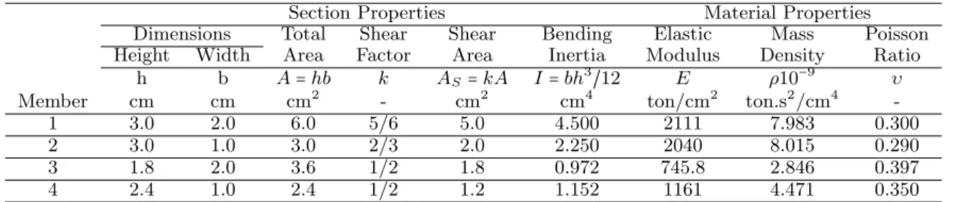
7.4 Robotic handler comprising Timoshenko beam members
Bending Released
Rigid Offset M K
5
4 o
1 2
3 4
P
20
mm 70 mm
50 100mm
30
Skewed Edge
Static Load
Actuator
Figure 7 Robotic handler comprising Timoshenko beam members in a complex configuration: end force release, rigid offset, skewed edge, concentrated massM=2Kg, concentrated springK=200ton/mm, static
loadP=5ton that weakens the horizontal arm, different sections and different materials (see table
8): (1) Steel 4139, (2) Steel ASTM A-515, (3) Aluminum 2024-T6, (4) Titanium 6AI-4V.
Table 8 Section and material properties for the robotic handler of Fig. 7.
Section Properties Material Properties
Dimensions Total Shear Shear Bending Elastic Mass Poisson
Height Width Area Factor Area Inertia Modulus Density Ratio
h b A=hb k AS=kA I=bh3/12 E ρ10−9 υ
Member cm cm cm2
- cm2
cm4
ton/cm2
ton.s2
/cm4
-1 3.0 2.0 6.0 5/6 5.0 4.500 2111 7.983 0.300
2 3.0 1.0 3.0 2/3 2.0 2.250 2040 8.015 0.290
3 1.8 2.0 3.6 1/2 1.8 0.972 745.8 2.846 0.397
4 2.4 1.0 2.4 1/2 1.2 1.152 1161 4.471 0.350
Table 9 Natural frequencies [Hz] for the robotic handler of Fig. 7.
Mode VIGENE PANSYS= 0.0 tona Error [%] VIGENE PANSYS= 5.0 tona Error [%]
1 14.988 14.988 0.000 12.577 12.570 0.056
2 145.98 145.98 0.000 145.88 145.86 0.014
3 4695.2 4695.2 0.000 4673.6 4634.0 0.855
4 5484.3 5484.4 -0.002 5392.8 5386.6 0.115
5 10148. 10148. 0.000 10148. 10148. 0.000
a
8 CONCLUSIONS
This work consolidates the possibility of using an iterative process for extracting eigenvalues, without the compulsory use of the Wittrick-Williams algorithm [6, 10, 11, 14]. Ref.[4] gives more details of the reasons why such an algorithm has operational difficulties when dealing with models that incorporate the special effects of end release and rigid offset.
For the examples here presented, the results in Table 10 show how an iterative determinant search method, based on the improved DSM of section 4.2, can be more computationally efficient. In terms of CPU time, the power secant method is always faster than a bracketing method based on the Wittrick-Williams algorithm. Therefore, as a well-known fact [1], the secant method is faster than any suitable determinant tracing, bracketing or bisection method.
Table 10 CPU (Intel Core2 E7400 2.8 GHz) Time [s] for the examples of section 7.
Tablea Caseb
Wittrick Power
ANSYS Time
Williams Secant Ratios
WWc PSd FEMe WW/PS FEM/PS
4 Pinned- pinned beam 1.688 0.891 3.188 1.9 3.6
Clamped- free beam 1.968 0.906 2.844 2.2 3.2
5
Clamped-pinned beam 1.953 0.797 3.344 2.5 4.2
Pinned- pinned beam 1.750 0.812 5.406 2.2 6.7
Clamped- clamped beam 1.641 0.797 2.891 2.1 3.6
6 Three-column building 3.969 1.328 3.188 3.0 2.4
7 Two-storey building 5.157 1.641 3.219 3.1 2.0
9 Robotic handler 4.625 1.625 2.859 2.8 1.8
a
Previous table with natural frequency results; b
For all the cases, the first 20 natural frequencies were calculated; c
Bracketing method based on the Wittrick-Williams algorithm which uses the classical DSM; d
Iterative secant method using the improved DSM; e
Subspace iteration method.
For CPU time comparison with FEM solutions, it must be considered that the FEM models, in general, cannot give accurate results unless fine meshes are employed. In the example of Fig 7, for instance, more than 240 beam elements were necessary in order to achieve a good accuracy. Having this in mind, Table 10 shows that the power secant method can be faster than the subspace iteration method [1] employed by the ANSYS program. When compared with FEM, however, the main advantage of the power secant method based on the improved DSM is the capability to find exact solutions that do not depend on the mesh refinement.
Finally, it must be emphasized that the Wittrick-Williams algorithm must use the classical formulation for the DSM while the power secant method must use the improved formulation as defined in section 4.2. As an additional advantage, the improved DSM preserves any local mode shape for which the nodal displacement vector Qo is null. Any other method based on
ill-conditioned. Moreover, using an inverse vector iteration method based on the improved DSM, it is possible to detect all the distinct mode shapes even when repeated natural frequencies exist.
References
[1] K. Bathe. Finite Element Procedures. Printice-Hall, New Jersey, 1996.
[2] R.D. Blevins. Formulas for Mode Shape & Natural Frequency. Krieger, Malabar, Florida, 1979.
[3] C.A.N. Dias. Computational system for dynamic analysis of in-plane beam structures. published on line in http://www.gmsie.usp.br.
[4] C.A.N. Dias and M. Alves. A contribution to the exact modal solution of in-plane beam structures.Journal of Sound and Vibration, 328(4-5):586–606, 2009.
[5] W.P. Howson and F.W. Williams. Natural frequencies of frames with axially loaded timoshenko members. Journal of Sound and Vibration, 26(4):503–515, 1973.
[6] S. Ilanko and F.W. Williams. Wittrick-Williams algorithm proof of bracketing and convergence theorems for eigen-values of constrained structures with positive and negative penalty parameters.International Journal for Numerical Methods in Engineering, 75:83–102, 2008.
[7] L. Majkut. Free and forced vibrations of timoshenko beams described by single difference equation. Journal of Theoretical and Applies Mechanics, 47(1):193–210, 2009.
[8] J.F. Martins. Rotatory inertia and shear force effects on the natural frequencies and dynamic response of framed structures. PhD thesis, Engineering School of S˜ao Carlos, University of S˜ao Paulo, Brazil, 1998.
[9] F.W. Williams, D. Kennedy, and M.S. Djoudi. Exact determinant for infinite order FEM representation of a Tim-oshenko beam-column via improved transcendental member stiffness matrices. International Journal of Numerical Method in Engineering, 59:1355–1371, 2004.
[10] F.W. Williams, S. Yuan, K. Ye, D. Kennedy, and M.S. Djoudi. Towards deep and simple understanding of the transcendental eigenproblem of structural vibrations. Journal of Sound and Vibration, 256(4):681–693, 2002.
[11] W.H. Wittrick and F.W. Williams. A general algorithm for computing natural frequencies of elastic structures.
Quarterly Journal of Mechanics and Applied Mathematics, 24:263–284, 1971.
[12] J-S. Wu and D-W. Chen. Free vibration analysis of a Timoshenko beam carrying multiple spring-mass systems by using numerical assembly technique.International Journal of Numerical Method in Engineering, 50:1039–1058, 2001.
[13] C-D. Yuan and W-H. Chieng. Method for finding multiple roots of polynomials. Computers and Mathematics with Applications, 51:605–620, 2006.
APPENDIX A. SIMPLY SUPPORTED RAYLEIGH BEAM UNDER AXIAL LOAD
In the case of disregarding shear deflection (s=0⇒ξ =1 ; η =randfT =∞), the problem
possesses an analytical solution that does not require the application of iterative numerical processes. By applying the boundary conditions in the functions that regulate the transverse displacements (7) and bending moments (10), respectively given by:
ϕv(x)=CS¯ T(x)+DC¯ T(x)+ES¯ H(x)+F C¯ H(x) (A.1)
ϕF(x)=−MT[CS¯ T(x)+DC¯ T(x)]+MH[ES¯ H(x)+F C¯ H(x)] (A.2)
we have :
a) Null transverse displacement atx=0
ϕv(0)=CS¯ T(0)+DC¯ T(0)+ES¯ H(0)+F C¯ H(0)=D¯ +F¯=0 (A.3)
b) Null bending moment atx=0
ϕF(0)=−MT[CS¯ T(0)+DC¯ T(0)]+MH[ES¯ H(0)+F C¯ H(0)]=
=−MTD¯+MHF¯=0
(A.4)
such that from Eq.s (A.3) and (A.4) it results that: ¯D=F¯ =0. c) Null transverse displacement at x=L
ϕv(L)=CS¯ T(L)+DC¯ T(L)+ES¯ H(L)+F C¯ H(L)=
=CS¯ T(L)+ES¯ H(L)=0 (A.5)
d) Null bending moment atx=L
ϕF(L)=−MT[CS¯ T(L)+DC¯ T(L)]+MH[ES¯ H(L)+F C¯ H(L)]=
=−MTCS¯ T(L)+MHES¯ H(L)=0
(A.6)
As the transition frequency is infinity, we have SH(L)≠ 0. Hence, Eq.s (A.5) and (A.6) are simultaneously satisfied if ¯E = 0 and ST(L) = 0, being ¯C ≠ 0 and arbitrary. Thus, the non-trivial solutions are obtained from:
ST(L)=sin(βTL)=sin(αT)=0⇒αT =iπ for i=1,2,3, ...,∞ (A.7)
It can be observed that the result of Eq. (A.7) is independent of the parametersr, s andp, respectively defined by Eqs. (12), (13) and (14), in a manner that it is also valid for any case of simply supported Timoshenko beam. The difference for the simply supported Euler-Bernoulli beam, with no axial loading, resides in the way by which the eigenvalues αT =iπ lead to the
natural frequencies. For an unloaded Euler-Bernoulli beam, with r =s =p =0, the solution simplifies to Ω=(iπ)2.
In order to use the known αT, however, the Rayleigh beam (p≠0 andr≠0) requires some
ξ=1 and η=r, it follows thatδ2=4Ω2and ¯∆=p2
+r2Ω2. So that, using (21) and (23), after
the following deduction:
2α2T =(∆¯2
+δ2)1/2+∆¯ ⇒(2α2T−∆¯) 2=∆¯2
+δ2⇒4α2T(α 2
T −∆¯)=δ 2
⇒
4α2T(α2T−p2−r2Ω2)=4Ω2⇒4α2T(α 2 T −p
2)=4(1
+r2α2T)Ω 2
for the non-dimensional frequency we may write :
Ω=αT √
α2 T−p2/
√
1+r2α2T (A.8)
Thus, usingαT =iπin Eq. (A.8), as well as the expressions (11), (14) and (17), the natural
frequencies are given by:
ωi[rad/s]=(iπ) √
(iπ)2
+P L2/EI √
EI/mL4/√1
+r2(iπ)2 (A.9)
By converting Eq. (A.9) for frequencies in Hz and by using the Euler buckling load (PCR=
π2EI/L2 ), we can finally write:
fi[Hz]=iπ √
i2
+P/PCR √
EI/mL4/√1
APPENDIX B. OVERFLOW LIMITING FREQUENCIES B.1 Limiting frequency (Ωlim 1) due to ∆¯
Observing Eq. (24), the condition:
¯
∆(ω)=p2+η2Ω2(ω)≤Rmax (B.1)
results in the following limit for the non-dimensional frequency:
Ω(ω)≤Ωlim 1= √
Rmax−p2/η (B.2)
B.2 Limiting frequencies (Ωlim 2 , Ωlim 3 and Ωlim 4) due to ∆˜
The expression (23) for ˜∆ can be viewed in the following form:
˜
∆2=A˜Ω4+B˜Ω2+p4 (B.3)
where
˜
A=(r2ξ2−s2)2≥0 (B.4)
˜
B=4+2p2(r2ξ2−s2) (B.5)
From this, three possible limits for the non-dimensional frequency can occur:
1. A.˜Ω4≤Rmax⇒Ω(ω)≤Ωlim 2=(Rmax/A˜)1/4 (B.6)
2. ∣B˜∣Ω2≤Rmax⇒Ω(ω)≤Ωlim 3=R1max/2 / √
∣B˜∣ (B.7)
3.
˜ AΩ4
+B˜Ω2+p4≤Rmax⇒ ⇒Ω(ω)≤Ωlim 4={(−B˜/2 ˜A)+
√
Rmax−p4/ √
˜
A}1/2 (B.8)
B.3 Limiting frequency (Ωlim 5) due to hyperbolic functions
If the current frequency is greater or equal to transition one (f ≥fT), overflow in the hyperbolic
functions will not occur because αH, according to Eq. (22), is purely imaginary number. In
contrast, (f < fT ⇒ δ2 > 0 ⇒ ∆˜ > ∆)¯ αH is real and must be lower than the following
computational limit:
αlim=acosh(Rmax)=ln(2)+ln(Rmax)≈ln(Rmax) (B.9)
Thus, using Eqs. (22), (24), (B.4) and (B.5), from the condition αH ≤αLim, we arrive at: √
˜ AΩ4
+B˜Ω2+p4−p2−η2Ω2≤2ξ2α2lim (B.10)
Case 1 Ifr2>0 ands2=0
1.1) Ifr2≥1/α2lim so
Ωlim 5=Rmax (B.11)
1.2) Ifr2<1/α2 lim so
Ωlim 5=αlim √
(α2
lim+p2)/(1−r2α 2
lim) (B.12)
Case 2 Ifr2=0 ands2>0
2.1) Ifs2≥1/αlim2 and p2≤1/4s2 ors2≤1/α2lim and p2≥1/4s2 so
Ωlim 5=Rmax (B.13)
2.2) Ifs2>1/α2
lim and p
2>1/4s2 ors2<1/α2
lim and p
2<1/4s2 so
Ωlim 5=2αlim √
(ξ2α2
lim+p2)/(s2α 2
lim−1)/(4s2p2−1) (B.14)
Case 3 Ifr2>0 ands2>0 so
Ωlim 5=Rmax (B.15)
Case 4 Ifr2=0 ands2=0 so
Ωlim 5=αlim √
α2
lim+p2 (B.16)

![Table 3 Natural frequencies [Hz] for a simply supported Euler-Bernoulli beam under axial load: L = 10 cm;](https://thumb-eu.123doks.com/thumbv2/123dok_br/18884363.423469/18.892.160.786.355.523/table-natural-frequencies-simply-supported-euler-bernoulli-axial.webp)
![Table 5 Natural frequencies [Hz] for the single Timoshenko beam of Wu-Chen [12]: L = 40 in; E = 3e7 psi;](https://thumb-eu.123doks.com/thumbv2/123dok_br/18884363.423469/19.892.83.771.164.324/table-natural-frequencies-hz-single-timoshenko-beam-chen.webp)
![Table 6 Natural frequencies [Hz] for the three-column building of Fig. 5: E = 78.0 Gpa; v = 0.33; ρ = 2500 Kg/m 3 ; A = 0.04 m 2 ; A S = 0.85A; I = 1.3333e − 4 m 4 .](https://thumb-eu.123doks.com/thumbv2/123dok_br/18884363.423469/20.892.314.628.163.360/table-natural-frequencies-hz-column-building-fig-gpa.webp)
![Table 10 CPU (Intel Core2 E7400 2.8 GHz) Time [s] for the examples of section 7.](https://thumb-eu.123doks.com/thumbv2/123dok_br/18884363.423469/22.892.148.798.387.625/table-cpu-intel-core-ghz-time-examples-section.webp)
