Abstract
The Modified Global Green's Function Method (MGGFM) is an integral technique that is characterized by good accuracy in the evaluation of boundary fluxes. This method uses only projections of the Green's Function for the solution of the discrete problem and this is the origin of the term 'Modified' of its name. In this paper the local strategy for calculating the projections of Green's function using de Finite Element Method (FEM) are detailed. The numerical examples show some aspects of the method that had not yet been observed andgoodresults for the flux in all nodes of the mesh.
Keywords
MGFM, MLGFM, MGGFM, local formulation, accurate fluxes.
The Local Formulation for the Modified
Green’
s Function Method
1 INTRODUCTION
The Modified Green s Function Method (MGFM) is an integral method that is characterized
mainly by the following factors:
1 - Contrary to the BEM (Boundary Element Method) and the Trefftz Method, this method does not use an analytical fundamental solution and/or a Green s function;
2 - Only pro‘ections of the Green s Function (denoted by GFp from now on) are required in the calculations. These projections can be calculated with appropriate numerical techniques. The Finite Element Method (FEM) is an interesting technique to obtain the discrete values for the GFp because they do not use fundamental solutions and/or Green s Functions. However, it is necessary to use an additional operator, N+, prescribed on the boundary by the user in order to avoid the singularity of the final system of equations;
3 - Precise values for the boundary generalized fluxes; and
Renato Barbieri a
Roberto Dalledone Machado b
a UDESC
[email protected] b UFPR
http://dx.doi.org/10.1590/1679-78251281
Latin American Journal of Solids and Structures 12 (2015) 883-904
placements) are identical to the FEM results. Therefore, all measures of the errors based on the displacements of the FEM also apply to the MGFM.
Using the FEM as a numerical method to obtain the discrete values for the GFp at least two approaches are possible: the global and the local formulations.
The global approach (MGGFM) is the formulation that has been most used by several authors in the last two decades and its implementation has been extensively studied. Therefore, this will not be shown in this paper. In this global formulation the auxiliary problems used to calculate the GFp are solved after the assembly of all elements of the mesh and one additional differential operator N+ is preferably prescribed at the boundary nodes with homogeneous Dirichlet boundary conditions. The time spent to calculate the GFp is higher than the conventional finite element calculations and the good flux convergence is observed only at the boundary nodes. The following works are examples of this approach: membranes, Barcellos and Silva (1987); Mindlin´s plate, Barbieri and Barcellos (1991, 1993); singular potential, Barcellos and Barbieri (1991); h and p convergence, Filippin et al. (1992); semi-thick shell, Barbieri et al. (1993), non-homogenous po-tentials problems, Barbieri and Barcellos (1993); subregions, Barbieri et al. (1994), laminated plates, Machado et al. (1994, 2008, 2012); 3D elasticity, Meira Jr. et al. (1995) and mathematical formulation, Barbieri et al. (1998,b).
Using the local formulation (MLGFM) the GFp are obtained in each element of the finite el-ement mesh. The additional operator N+ is prescribed by the user at the element boundary nodes. The advantages of this formulation are the accurate flux at all nodes of the mesh and the reduction of processing time of the analysis compared with the global formulation.
This paper was organized in a way of providing the reader with just a review of the MGFM basics mathematical concepts and showing the details of the MLGFM implementation.
The examples solved with the local approach (MLGFM) included in the text show accurate results for the flux in all nodes of the mesh. The solution of the one-dimensional Burgers equation (nonlinear problem) using the Hopf-Cole transformation is another application of this local tech-nique to approximate the GFp due to the flux accurate evaluation at all nodes of the mesh.
The examples solved with the global approach (MGGFM) show new results obtained with high-order (p=4) elements for two-dimensional singular potential problem and new observations for the h and p convergences for regular potential problems.
2 MGFM: BASIC CONCEPTS AND ITS NUMERICAL IMPLEMENTATION
The mathematical aspects shown in this section and all procedures for the numerical implementa-tion of the MGFM have been previously described by Barcellos and Silva (1987), Silva (1988) and Barbieri et al. (1998). Small reviews of the main concepts of this method are included in the text to show some details that will be discussed throughout this paper.
The u(Q) solution for the linear equation system
(Q)
Q
)Q ( b
Latin American Journal of Solids and Structures 12 (2015) 883-904 With boundary conditions properly prescribed can be obtained using the following integral equa-tion:
(P,Q) (P)d [ (p,Q)] (p)d (p,Q)[ (p)]d
) Q
( G tb N*G tu G Nu
u t (2)
where P and Q are domain points, (P,Q); p and q are boundary points, (p,q); N and N* are the Neumann operators associated with the differential operator A and with its adjunct operator A*, respectively; b(P) is the generalized force vector and G(,) is a fundamental
solu-tion.
Adding and subtracting the quantity G(p,Q)t[Nu(p)][NG(p,Q)]tu(p)in Eq. (2) we obtain:
(P,Q) (P)d [( ) (p,Q)] (p)d (p,Q)[( ) (p)]d )
Q
( G tb N N G tu G t N N u
u * (3)
where N+ is an additional operator prescribed by the user. The choice and specification of this operator was detailed by Barbieri et al. (1998a).
If it is prescribed the boundary condition (N*+N+)G(p,Q)=0, the function G(,) becomes a
Green Function and the solution for u(Q) can be rewritten as follows:
Q d ) p ( ) Q , p ( d ) P ( ) Q , P ( ) Q( G tb G tF
u (4)
q d ) p ( ) q , p ( d ) P ( ) q , P ( ) q( G tb G tF
u (5)
where F(p)=(N+N+)u(p).
After the conventional approximations of the variables u(Q), b(P) and F(p) with the finite elements or the boundary elements interpolations, the process of residues orthogonalization with
the Galer’in s method of Eq.(4) results:
t d{uD}
tG(P,Q)t
dd{b}
tG(p,Q)t
dd{f}
(6)
where u(Q)[]{uD}, b(P) []{b}, F(p) []{f}, [] being the set of interpolation functions of the domain (base of the finite elements subspace) and [] is the set of interpolation functions of the boundary (base of the boundary elements subspace). The vector components {uD}, {b} and {f} represent nodal values for the generalized displacement, for the generalized body forces and for the reactions on the boundary, respectively.
Eq.(6) can be rewritten as:
td{uD}Gd(P)t
d{b}Gd(p)t
d{f}
(7)
where Gd() represents the GFp on the subspace generated by the finite element basis,
(P,Q) d
) P
( t tG t
Gd and
(p,Q) d
) p
( t tG t
Latin American Journal of Solids and Structures 12 (2015) 883-904
Repeating the same procedure for Eq.(5), we have:
t d{ub}
t
G(P,q)t
dd{b}
t
G(p,q)t
dd{f}
(8)
where u(q)= []{ub}, [] is the basis of the boundary elements subspace (trace of []) and {ub} is the displacements vector on the boundary. According to the convenience, the forces on the boundary F(p) can be interpolated using [][].
Again, it is convenient to rewrite Eq.(8) in the following way:
t d{ub}
Gb(P)t
d{b}
Gb(p)t
d{f}
(9)
where Gb() represents the GFp on the subspace generated by the boundary elements basis,
(P,q) d
) P
( t tG t
Gb and
(p,q) d
) p
( t tG t
Gb . The numerical calculation of the
Green s Function pro‘ections Gd() and Gb() is carried out by solving the following associated
problems, Barcellos and Silva (1987):
Problem 1: Find Gd(P) :
(p) 0 p ,P
) P ( ) P ( d * d * G ) N (N G A (10)
Problem 2: Find Gb(P) :
) (p) (p) p ,P ( 0 ) P ( b * b * G N N G A (11)
Finally, after calculating the nodal values of Gd() and Gb(), the nodal values for u(Q) and F(p)
are obtained solving Eqs.(7) and (9).
3 THE MLGFM FORMULATION
The formulation shown in sequence is an extension of the concepts used by Barbieri et al. (1994) and Barbieri and Muñoz (1998) for subregions. A one dimensional problem modeled with linear finite elements is taken as an example to better understand the concepts of the local formulation of the method. Thus, when N+=0 the finite element equations for the problems (10) and (11) can be written as:
Latin American Journal of Solids and Structures 12 (2015) 883-904 To obtain discrete values of the GFp for each node of the element it is necessary to prescribe the additional operator N+0 because the system of Eq (12) is singular. Figure 1 shows the scheme used in this work to prescribe the additional operator N+ at the element boundary nodes.
Figure 1: Boundary Conditions and the additional operator N+ for the local formulation.
The scheme illustrated in Figure 2 shows the boundary conditions and the loading used for the discrete calculation of Gd() and Gb() for each element. The GFp is calculated solving the
follow-ing system of equations:
2 , 2 1 , 2 2 , 1 1 , 1 2 , 2 d 1 , 2 d 2 , 1 d 1 , 1 d 2 , 2 b 1 , 2 b 2 , 1 b 1 , 1 b 0 2 , 2 1 , 2 2 , 1 0 1 , 1 M M M M 1 0 0 1 G G G G G G G G k k k k k k (13)
where M,ij
i(x)j(x)dx.4 THE FINAL SYSTEM OF EQUATIONS
Barcellos and Silva (1987) have shown that Eq. (7) can be rewritten in the following matricial form:
I{uD}
Gb
f
Gd
b (14)where [Gc] and [Gd] are matrices of discrete values of the GFp obtained by solving equations (10)
and (11), respectively.
The assembled final system of equation is obtained considering the potencial (or displace-ment) continuity and the flux balance for the internal nodes of the mesh. The final system of equations is solved after imposing the boundary conditions of the problem. At the end of this step all nodal values for {u} and {f} are known. At this point, we have to remember that ficti-tious fluxes were added when prescribing the additional operator N+u=k0u at all internal nodes
of the mesh during the evaluation of the GFp. Therefore, the correct flux is obtained through subtraction of the additional part k0uj for any internal node j of the mesh.
-k0 k0 -k0 k0
Latin American Journal of Solids and Structures 12 (2015) 883-904
(a) Problem 1.
(b) Problem 2.
Figure 2: Loads and boundary conditions for the local formulation.
5 RESULTS
If not mentioned, the flux results of the FEM are obtained using the global smoothing technique described by Hinton and Campbell (1974) and using Lagrangian elements.
5.1 One-dimensional Wave Equation
Problem: Find the solution u(x) for:
1 x 0 0
x ) x ( u dx
) x ( u d
2 2
(15)
with boundary conditions: u(0)=0 and du(1)/dx=0. The analytical solution for this problem is u(x)= sin(x)/cos(1) – x.
Homogeneous finite element meshes (N elements with degree p=1 to p=4) were used to
ob-tain the GFp and the additional operator N+u=1.u was prescribed according to the scheme
illustrated in Figure 1. The objective of this analysis is to evaluate the flux convergence at all nodes of the mesh and compare these results with the errors obtained with the FEM.
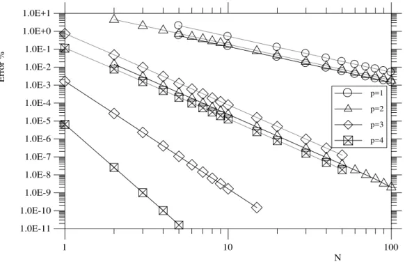
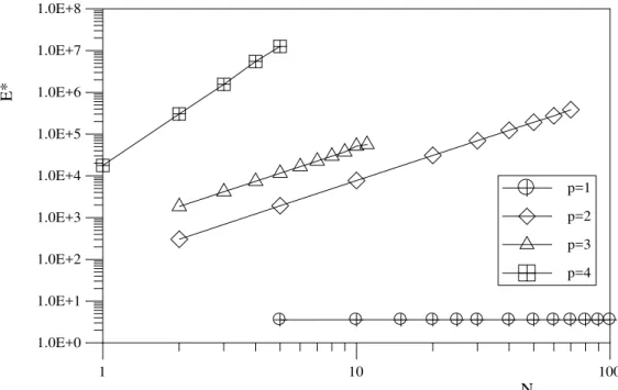
In Figure 3 are shown the results obtained for the h convergence of the flux at x=0 and in Figure 4 are shown the curves for the relative error, E*=E%FEM/E%MLGFM. All curves of these
figures can be approximated with functions of the type, E*C(p)Nm, where C(p) and m are two constants that depend on the degree of the element. The adjusted values for these two parame-ters are shown in Table 1.
1
1(x)
k0 -k0
2
2(x)
k0 -k0
1 2
2 1
k0
1(x)=1
-k0
1 2
2(x)=1
-k0
Latin American Journal of Solids and Structures 12 (2015) 883-904 Contrary to expectations, the flux results obtained with the MLGFM using the linear element are close to the FEM results and with similar rates of convergence. For higher order elements (p2) the results obtained with the MLGFM are always better than those obtained with the FEM and with higher convergence rates. Whereas the results MLGFM have convergence rate with a value close to m-2p, the results of the FEM present convergence rates near to m-2 for linear and quadratic elements and m-4 for cubic and fourth order elements. More detailed analy-sis on h and p convergence of finite element solutions for the problem can be found in the litera-ture, for example Ihlenburg (1998), Bouillard (1999), Ihlenburg and Babuska (1997) and Bouillard and Ihlenburg (1999).
In Tables 2 and 3 are shown the results for the flux at x=0 obtained with a homogeneous mesh with 5 elements. The first observation to be made is that the flux errors obtained with MLGFM are approximately constant for all nodes of the mesh and the Neumann condition is automatically satisfied when the boundary condition is imposed for the solution of the final system of equations. Moreover, the error in the flux obtained with the FEM varies from node to node and the Neu-mann boundary condition at x=1 is only achieved when h0.
1 10 100
N 1.0E-11
1.0E-10 1.0E-9 1.0E-8 1.0E-7 1.0E-6 1.0E-5 1.0E-4 1.0E-3 1.0E-2 1.0E-1 1.0E+0 1.0E+1
E
rr
or
%
p=1
p=2
p=3
p=4
Latin American Journal of Solids and Structures 12 (2015) 883-904
Figure 4: Relative error for the flux du(0)/dx, E*=E%FEM/E%MLGFM.
.
Element order
MLGFM FEM E*
C(p) m C(p) m C(p) m
p=1 14.0043 -1.9981 49.9117 -1.9977 3.564 2.973110-4
p=2 0.2404 -4.0123 17.8421 -1.9957 74.225 2.0166
p=3 1.639910-3 -5.9876 0.7580 -3.9911 456.966 2.0049
p=4 6.590410-6 -8.0074 0.7580 -3.9911 17751.700 4.0774
Table 1: Fitted values for C(p) and m.
x p=1 p=2 p=3 p=4
0 1.99710-2 0.72110-3 2.06210-4 1.24010-5
0,2 2.03110-2 7.39010-3 2.11310-4 1.27110-5
0,4 2.15310-2 8.02210-3 2.29310-4 1.37910-5
0,6 2.46310-2 9.60310-3 2.74510-4 1.65110-5
0,8 3.48710-2 1.47810-2 4.22310-4 2.53910-5
Table 2: FEM results for the Error % in du(x)/dx (N=5).
1 10 100
N
1.0E+0 1.0E+1 1.0E+2 1.0E+3 1.0E+4 1.0E+5 1.0E+6 1.0E+7 1.0E+8
E
*
p=1
p=2
p=3
Latin American Journal of Solids and Structures 12 (2015) 883-904
x p=1 p=2 p=3 p=4
0 5.60410-3 3.75610-6 1.07410-9 1.60510-12
0,2 5.59110-3 3.74810-6 1.07210-9 1.81410-12
0,4 5.55510-3 3.72410-6 1.06510-9 1.89110-12
0,6 5.49310-3 3.68210-6 1.05310-9 1.93610-12
0,8 5.40610-3 3.62410-6 1.03610-9 2.26310-12
Table 3: MLGFM results for the Error % in du(x)/dx (N=5).
To conclude this example, other two results are shown in Table 4 and Figure 5. The results in Table 4 show the values of flux errors for all nodes of the ends of the elements (N=10, p=2) and the results of Figure 5 illustrate the errors in the potential and flux obtained with the MLGFM (N=20, p=2). It is noteworthy the fact that the errors for the flux are lower than the errors for the potential in Figure 5.
x Analitic FEM Error % MLGFM Error % E*
0 0,8508157177 0.85235299 0.181 0.8508155176 2.35210-5 7695.57
0,1 0,8415693483 0.84309894 0.182 0.8415691505 2.35010-5 7744.68
0,2 0,8139226266 0.81542926 0.185 0.8139224357 2.34510-5 7889.12
0,3 0,7681517897 0.76962041 0.191 0.7681516100 2.33910-5 8165.88
0,4 0,7047141646 0.70613011 0.201 0.7047140004 2.33010-5 8626.60
0,5 0,6242435991 0.62559272 0.216 0.6242434543 2.31910-5 9314.35
0,6 0,5275441284 0.52881300 0.241 0.5275440068 2.30510-5 10455.53
0,7 0,4155819418 0.41675814 0.283 0.4155818467 2.28810-5 12368.88
0,8 0,2894757283 0.29054898 0.371 0.2894756626 2.26910-5 16339.79
0,9 0,1504854995 0.15145373 0.643 0.1504854657 2.24610-5 28628.67
1,0 0 0.00090388 - 0 0 -
Latin American Journal of Solids and Structures 12 (2015) 883-904
Figure 5: Errors for potential and flux (N=20 and p=2).
5.2 One-dimensional Burgers Equation
The one-dimensional Burgers equation can be written as follows:
) t , x ( f x ) t , x ( u x ) t , x ( u ) t , x ( u t ) t , x ( u 2 2 (16)
where u(x,t) denotes the variable of interest, is a positive constant and its value and physical interpretation depends on the problem being studied and f(x,t) is a source term. There are no analytical solutions for the Burgers equation, but for some combinations of boundary conditions
and initial conditions it is possible to obtain the exact solution usually written as infinite series
.
For >0 values, it is assumed that there is a function (x,t) such that u(x,t)=(x,t)/x and its derivatives are limited for all (x,t). Substituting this transformation of variables in Eq.(16) and employing the Hopf-Cole transformation (x,t)=-2ln((x,t)), Cole (1951), then u(x,t) is obtained with the following expression) t , x ( x / ) t , x ( 2 x ) t , x ( ) t , x ( u (17)
and the non-linear equation (16) becomes linear for (x,t), i.e:
2 2 x ) t , x ( t ) t , x ( (18)
Employing the Crank-Nicolson rule to approximate the time derivative and writing the Eq. (18) for the time (n+1)t we have:
n n 2 1 n 2 1
n t( 1)
x
t
(19)
0.00 0.20 0.40 0.60 0.80 1.00
Latin American Journal of Solids and Structures 12 (2015) 883-904 which is a one-dimensional linear differential equation with constant coefficients and time-varying excitation.
However, although the Hopf-Cole transformation probably makes the solution of the Burgers equation less laborious, one of the inconveniencies of this method is that the calculation of the partial derivative of the auxiliary function (x,t) with respect to x must be precise to obtain the correct value of u(x,t). Obtaining an accurate value for the spatial derivatives has always been the weak point of many numerical methods used for solving this type of problem.
To verify the efficiency of MLGFM in solving this type of problem, the procedure described above was used in the solution of the Burgers equation with initial conditions given by u(x,0)=sin (x), x[0,1] and boundary conditions u(0,t)=u(1,t)=0, t[0,T]. Although an analytical solution exists for this problem it is written in the form of a series with infinite terms and according to Kutluay at al. (1999) 'It is known that the exact solutions for <0.01 fail because of the slow convergence of the infinite series'.
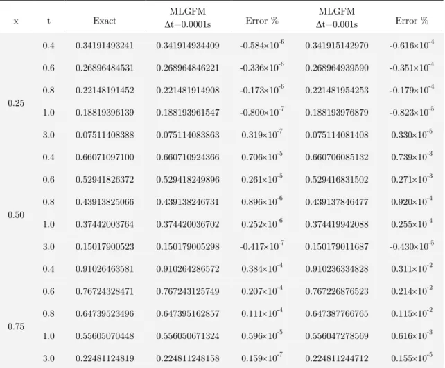
The results shown in the sequence were obtained from the MLGFM using homogeneous meshes with 800 quadratic elements (to compare with others results) for the calculation of the GFp and =0.01. The analytical solution for some instants of time is shown in Figure 6 and we note that some curves have a strong gradient around x=1. The values shown in Table 5 illustrate the influence of the t value in the accuracy of the method. In Figure 7 are carried out compara-tive studies with literature data. As expected, the errors obtained with the MLGFM are better than those obtained by other techniques due the fact that the partial derivatives of (x, t) with respect to x are better evaluated by this method.
Figure 6: Analytical solution u(x,t) with =0.01.
0.0 0.1 0.2 0.3 0.4 0.5 0.6 0.7 0.8 0.9 1.0
x
0.0 0.1 0.2 0.3 0.4 0.5 0.6 0.7 0.8 0.9 1.0
u(
x,
t)
t=0.4s
t=0.6s
t=0.8s t=1.0s
t=3.0s
Latin American Journal of Solids and Structures 12 (2015) 883-904
x t Exact MLGFM t=0.0001s Error % MLGFM t=0.001s Error %
0.25
0.4 0.34191493241 0.341914934409 -0.58410-6 0.341915142970 -0.61610-4
0.6 0.26896484531 0.268964846221 -0.33610-6 0.268964939590 -0.35110-4
0.8 0.22148191452 0.221481914908 -0.17310-6 0.221481954253 -0.17910-4
1.0 0.18819396139 0.188193961547 -0.80010-7 0.188193976879 -0.82310-5
3.0 0.07511408388 0.075114083863 0.31910-7 0.075114081408 0.33010-5
0.50
0.4 0.66071097100 0.660710924366 0.70610-5 0.660706085132 0.73910-3
0.6 0.52941826372 0.529418249896 0.26110-5 0.529416831502 0.27110-3
0.8 0.43913825066 0.439138246731 0.89610-6 0.439137846477 0.92010-4
1.0 0.37442003764 0.374420036702 0.25210-6 0.374419942088 0.25510-4
3.0 0.15017900523 0.150179005298 -0.41710-7 0.150179011687 -0.43010-5
0.75
0.4 0.91026463581 0.910264286572 0.38410-4 0.910236334828 0.31110-2
0.6 0.76724328471 0.767243125749 0.20710-4 0.767226876523 0.21410-2
0.8 0.64739523496 0.647395162857 0.11110-4 0.647387766765 0.11510-2
1.0 0.55605070448 0.556050671324 0.59610-5 0.556047278569 0.61610-3
3.0 0.22481124819 0.224811248158 0.15910-7 0.224811244712 0.15510-5
Table 5: Influence of the t value in the MLGFM solutions (=0.01, p=2 and N=800).
0.0 1.0 2.0 3.0
t 1.0E-8
1.0E-7 1.0E-6 1.0E-5 1.0E-4 1.0E-3 1.0E-2 1.0E-1 1.0E+0 1.0E+1
E
rr
or
%
MLGFM Kutluay et al. (2004) Kutluay et al. (1999) Kutluay et al. (1999) Özis et al. (2005) Kadalbajoo et al. (2006)
Latin American Journal of Solids and Structures 12 (2015) 883-904
5.3 Two-dimensional Singular Potential
Problem: Find the solution u(r,) for:
u(r, ) 0 (r, ) (20)
3 2 2 / 1 1 ) , r ( 0 ) , r ( u ) , r ( ) 2 / cos( r ) , r ( u ) , r ( 0 n ) , r ( u (21)
where ={(r,):0r1;0}; 1={(r,):0r1;=0}; 2={(r,):r=1;0}
and 3={(r,):0r1;=}. This is a problem with analytical solution equal to
) r cos( /2); (r, ) ,
r (
u 1/2 and presents singularity at r=0.
Fourth order finite elements (p=4) are used to discretize the domain according to the pattern shown in Figure 8a. Since this is a singular problem, special finite elements (obtained from the analytical behavior of the solution) were used around the singular point. These special elements are perfectly compatible with the Lagrangian elements and approach u(r,) with behavior r for 01. The formulation of the special elements was detailed by Barbieri (2005) and its geometry is shown schematically in Figure 8b. The node 1 is always placed at the singular point and the other nodes are numbered counterclockwise and placed on the semicircle (or circle). The radius R of such semicircle is small enough to ensure that the singularity is quite well represented. The results of this work was obtained using a mesh with 12 subdivisions in the direction and ar-ranged in pg (geometric progression) subdivisions with ratio equal to 0.5 in the radial direction from r=0.5 to r=R=1.52587910-5 (shaded region in the Figure 8a).
(a) Finite Element Mesh
-1.00 -0.75 -0.50 -0.25 0.00 0.25 0.50 0.75 1.00 0.00
0.25 0.50 0.75 1.00
Latin American Journal of Solids and Structures 12 (2015) 883-904
(b) Singular element
Figure 8: Finite Element Mesh for evaluation of the GFp.
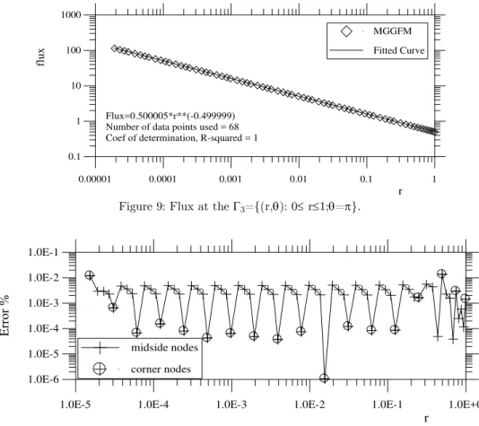
Contrary to observed results in other applications, Barcellos and Barbieri (1991) and Maldaner (1993), the oscillations of the flux results around the analytical solution are very small, even close to the singular point. For (r,) 3 the analytical expression for the flux is u(r,0)/n=0.5r-0.5
and the flux obtained with the MGGFM was u(r,0)/n0.500005r-0.499999, see Figure 9. Observ-ing the results for the flux of Figure 10 we note that the best values around the sObserv-ingular point were obtained at the inter-element nodes (boundary element mesh). Barcellos and Barbieri (1991) also observed this behavior with elements of lower order.
Figure 9: Flux at the 3={(r,): 0 r1;=}.
Figure 10: Error % for the flux at the nodes in 3={(r,): 0 r1;=}.
1.0E-5 1.0E-4 1.0E-3 1.0E-2 1.0E-1 1.0E+0
r
1.0E-6 1.0E-5 1.0E-4 1.0E-3 1.0E-2 1.0E-1
E
rr
or
%
midside nodes
corner nodes
y
6 2
3 4
2
1 R
x 5 6
Singularity
0.00001 0.0001 0.001 0.01 0.1 1 r 0.1
1 10 100 1000
fl
ux
MGGFM
Fitted Curve
Latin American Journal of Solids and Structures 12 (2015) 883-904
5.4 Two-dimensional Steady State Heat Transfer
Problem: Find the solution for:
u(r, ) 0 1 r 10;0 2 (22)
0 T ) u(10,
1000 T
) u(1,
e i
(23)
The analytical solution of this problem is:
i i e
i e
i ln(TR /TR )ln Rr T
) , r (
u (23)
with Re=10 and Ri=1. The radial flux u(r,)/r, calculated at r=Ri=1 is the parameter used in
this example for comparisons with the numerical results.
The global formulation of the MGGFM is used to solve this problem and, due to the charac-teristic of the analytical solution, only a circular sector (05/180) is modeled using only one element in the direction and N homogeneous elements in the radial direction with variable p
(p=2,…,p=8).
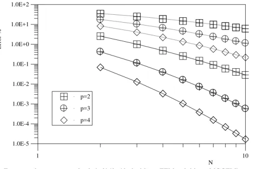
The curves plotted in Figure 11 show the h convergence for the radial flux u(1,)/r ob-tained with different elements (p=2, p=3 and p=4). Besides showing that the values obob-tained with the MGGFM are much better than the values of the FEM, these results show significant reduction of errors when increasing the order of the element (for both methods). The curves of Figure 12 show the relative errors, E*=Error%FEM/Error%MGGFM, obtained with the elements of
order 2, 3 and 4. A mathematical expression of type E*=C(p)Nm can be used to represent these errors and the fitted curves valid for N>4 are also shown in this figure.
Figure 11: h convergence for u(1,)/r (dashed line=FEM, solid line=MGGFM).
1 10
N 1.0E-5
1.0E-4 1.0E-3 1.0E-2 1.0E-1 1.0E+0 1.0E+1 1.0E+2
E
rr
or
%
p=2
p=3
Latin American Journal of Solids and Structures 12 (2015) 883-904
Figure 12: Results for E* (solid line=fit results, dashed line=numeric).
Figure 13: p convergence for u(1,)/r.
Finally, to complete this example, the problem being studied was again solved with homogeneous mesh with N=5 and p varying from 2 to 8. The results in Figure 13 show the p convergence for the radial flux u(1,)/r. The mathematical expression for the relative error, E*, obtained with these data was E*=3.44942e1.46107p with values varying from 64.08 for p=2 to 410941 for p=8.
2 3 4 5 6 7 8
p 1.0E-8
1.0E-7 1.0E-6 1.0E-5 1.0E-4 1.0E-3 1.0E-2 1.0E-1 1.0E+0 1.0E+1 1.0E+2
E
rr
or
%
Fit Results (FEM):
ln(Error%) = -1.27103*p + 5.31311
Coef. of determination, R-squared = 0.999394
Fit Results (MGGFM): ln(Error%)=-2.7321*p+4.07491
Coef. of determination, R-squared = 0.999978
FEM
MGGFM
1 10
N 1.0E+1
1.0E+2 1.0E+3 1.0E+4 1.0E+5
E
*
Fit Results for N>4: E*=2.745*N**1.883 p=2 E*=2.938*N**2.803 p=3 E*=5.962*N**3.319 p=4
p=2
p=3
Latin American Journal of Solids and Structures 12 (2015) 883-904
5.5 Two-dimensional Potential Problem
Find the solution u(x) for the equation:
1 y , x 1 )]
x 1 ( y ) y 1 ( x )[ 1 n 2 ( n 2
u 2n 2 2n 2n 2 2n
(24)
with n being an integer (n=5 in this example) and with homogeneous Dirichlet boundary condi-tions. This problem was solved by Barbieri et al. (1998) and he was once again solved with MGGFM to show new conclusions based on the results of the flux. Its analytical solution is u(x)=(1-x2n)(1-y2n) and the analytical flux at x=(1,0) is equal to -10.
Due to the problem´s symmetry, only a quarter of the domain is discretized with uniform fi-nite element meshes and their respective boundary meshes are employed for the evaluation of the GFp using the MGGFM, Figure 14.
(a) Domain (b) Additional Operator, k=1.
(c) Boundary Element mesh (p=2)
(d) 22 Finite Element mesh (p=2).
Figure 14: Problem discretization.
The curves of Figures 15 and 16 show the results for the h convergence (h=1/N). These curves can be fitted with equations of type 'Error%=C(p)hm(p)' and the values for C(p) and m(p) are shown in Table 10. From these results we note that while the rates of p convergence for the FEM grow with approximately constant rate, this same behavior does not happen for the results of the MGGFM where m(2)=3.861; m(3)=3.939; m(4)=5.879; m(5)=5.996 and m(6)=7.871.
This behavior is best visualized from the results of the p convergence to the flux in (1,0) illus-trated in Figure 17. The results of the FEM are always improved with increasing the order of the elements and this same behavior does not apply to the MGGFM results. However, the values for the relative error, E*, indicated in Table 10 show that for the same element, the results of MGGFM are always better than the results of the FEM.
2 2
x
Latin American Journal of Solids and Structures 12 (2015) 883-904
Figure 15: h convergente for u(1,0)/n (FEM).
Figure 16: h convergente for u(1,0)/n (MGGFM).
p FEM MGGFM E*
2 133.418h1.487 74.487h3.861 1.791h-2.374
3 107.662h2.585 40.597h3.939 2.652h-1.354
4 50.450h3.556 2.576h5.879 19.583h-2.324
5 17.876h4.680 1.726h5.996 10.389h-1.316
6 3.891h5.689 0.01999h7.871 194.669h-2.181
Table 10: Adjusted curves for the error% in u(1,0)/n and for the Relative Error, E*.
0.1 h 1.0
1.0E-6 1.0E-5 1.0E-4 1.0E-3 1.0E-2 1.0E-1 1.0E+0 1.0E+1 1.0E+2
E
rr
or
%
FEM
p=2
p=3
p=4
p=5
p=6
0.1 h 1.0
1.0E-9 1.0E-8 1.0E-7 1.0E-6 1.0E-5 1.0E-4 1.0E-3 1.0E-2 1.0E-1 1.0E+0 1.0E+1
E
rr
or
%
MGGFM
p=2
p=3
p=4
p=5
Latin American Journal of Solids and Structures 12 (2015) 883-904 Figure 17: p convergence for u(1,0)/n (solid line=MGGFM, dashed-line=FEM).
6 CONCLUSIONS
In this paper the local formulation for the MGFM was shown. With this formulation it is possible to obtain good results for the flux at all nodes of the mesh. The formulation shown was meant for one-dimensional problems. The extension of these concepts to two-dimensional and three-dimensional cases is still a topic under study.
In Example 5.1 the solution of the wave equation is displayed using the local formulation of the method and the results showed:
-good convergence for the flux in all nodes of the mesh for p> 1;
-Contrary to our expectations, for p=1 the flux results of the MLGFM are better than the results of the FEM, but with small difference;
-the MLGFM errors for the flux are approximately constant for all nodes of the mesh, and
-E * values indicate that the change of the quadratic element (p=2) for the cubic element (p=3) does not improve its rate of convergence.
Example 5.2 was directed to the solution of the Burgers equation. This is a nonlinear equa-tion and the Hopf-Cole transformaequa-tion and the Crank-Nicolson rule was used to obtain a discrete time linear problem. Local MGFM approach was used to solve this equation and the results show the influence of t on the accuracy of the method and the good convergence of the method for any instant of time.
1 p 10
1.0E-9 1.0E-8 1.0E-7 1.0E-6 1.0E-5 1.0E-4 1.0E-3 1.0E-2 1.0E-1 1.0E+0 1.0E+1 1.0E+2
E
rr
or
% MGFM h=1/2
Latin American Journal of Solids and Structures 12 (2015) 883-904
MGFM is displayed. The meshes used to solve this example were prepared with elements of fourth order (p=4) and using specific elements (singular) around the singular point. The results showed that:
- the quality of approximations of GFp influences the flux results;
- the approximation of F(p) with appropriate functions (singular) produce accurate results for the flux;
- no flux fluctuation around the singular point was observed.
Problems 5.4 and 5.5 were solved with MGGFM with the aim of showing some new observations on the flux convergence. More research is still needed on this topic to study the small reduction in error of the flux when odd elements are used to obtain the GFp.
In this paper the FEM was used to obtain GFp and for this reason the MGFM results were compared with the FEM results. Comparisons with flux results obtained with other techniques are still needed to extend the conclusions on the quality of the flux results shown in this paper.
Acknowledgments
The authors thank Professor Clovis Sperb de Barcellos, whose deep technical formation has been transmitted over a number of years of coexistence and friendship. The authors would also like to thank the Brazilian National Council for Research, CNPq, for the financial support.
References
Barbieri, R.; Barcellos, C. S. (1991). A Modified Local Green´S Function Technique for the Mindlin´s Plate Mod-el. In: XIII BEM Conference, Tulsa. Proceedings. Tulsa-USA, p. 551-565.
Barbieri, R.; Barcellos, C. S. (1993). Non-Homogeneous Field Potential Problems Solution by the Modified Local Green´s Function Method (Mlgfm). Engineering Analyis with Boundary Elements, UK, v.11, n.1, p. 9-15.
Barbieri, R.; Barcellos, C. S. (1993) - Mindlin´s Plate Solutions by the Mlgfm. In: BEM XV - International Con-ference on Boundary Element Method, 1993, Albuquerque,USA, v.2, p.149-164.
Barbieri, R.; Machado, R. D.; Filippin, C. G. and Barcellos, C. S. (1994). MLGFM – A Formulation for Sub-regions (in portuguese). In: XV CILANCE- Congresso Ibero Latino Americano de Métodos Computacionais para a Engenharia, Belo Horizonte. Anais do CILANCE. Belo Horizonte-MG, p.671-680.
Barbieri, R.; Muñoz, R. P. A; Machado, R. D. (1998) - Modified Local Green´S Function Method (Mlgfm). Part I: Mathematical Background And Formulation. Engineering Analysis with Boundary Elements (EABE), UK, v.2, n.22, p. 141-151.
Barbieri, R.; Muñoz, R. P. A.(1998) - Modified Local Green´s Function Method (Mlgfm). Part II: Application For Accurate Flux And Traction Evaluation. Engineering Analysis with Boundary Elements (EABE), UK, v.2, n. 22, p. 153-159.
Latin American Journal of Solids and Structures 12 (2015) 883-904 Barbieri, R. (2005) – MLGFM – Analysis of nodal flux superconvergence for higher order elements. Technical Report (in portuguese) CNPq Proc. 302809/2003-0.
Barbieri, R. (2013) – Convergence analysis of numerical solutions of Burger´s Equation by the Modified Local Green Function Method (MLGFM). Technical Report (in Portuguese). CNPq Proc. 302809/2009-0.
Barcellos, C.S.; Silva, L.H.M. (1987) - Elastic Membrane Solution by a Modified Local Green´s Function Method. (Ed. Brebbia, C.A. and Venturine, C.S.). Proc. Int. Conference on Boundary Element Technology, Comp. Mech. Publication, Southampton.
Barcellos, C. S.; Barbieri, R. (1991).Solution of Singular Potential Problems by the Modified Local Green´s Func-tion Method (Mlgfm). In: XIII BEM Conference, Tulsa-USA, p. 851-862.
Barcellos, C. S.; Barbieri, R.; Muñoz, R. P. A.; Meira Jr, A. D. (1995) - A Comparison of the Modified Local Green´s Function Method (MLGFM) and the Finite Element Method (FEM) for Some Problems In 3-D Elastici-ty. In: XVI CILANCE - Congresso Ibero Latino Americano de Métodos Computacionais para a Engenharia, Curi-tiba, p.80-89.
Cole, J.D. (1951). On a quasi linear parabolic equation occurring in aerodynamics, Quart. Appl. Math. 9:225–236.
Filippin, C. G.; Barbieri, R.; Barcellos, C. S. (1991). Numerical Results for h and p Convergences For The Modi-fied Local Green´S Function Method. In: VII Boundary Element Technology, Tulsa-USA, p. 887-904.
Frank Ihlenburg. Finite Element Analysis of Acoustic Scattering. Springer-Verlag New York, Inc., 1998.
F. Ihlenburg and I. Babuska (1997). Reliability of Finite Element Methods for the Numerical Computation Waves. Advances in Engineering Software 28, 417-424.
Hinton E.; Campbell, JS. (1974) - Local and global smoothing of discontinuous finite element functions using a least squares method. Int. J. Numer. Meth. Eng.;8 (3):461–80.
Kutluay, S, Bahadir, A.R.; Ozdes, A. - (1999) Numerical solution of one-dimensional Burger´s equation: explicit and exact-explicit difference methods, J. Comput. Appl. Math. 103, 251–261.
Kutluay, S; Esen, A; Dag, I; (2004) - Numerical solutions of the Burgers equation by the least-squares quadratic B-spline finite element method. Journal of Computational and Applied Mathematics 167, 21–33.
Machado, R.D.; Abdalla Fo, J.E.; Silva, M. P.; Stiffness loss of laminated composite plates with distributed damage by the modified local Green s function method. Composite Structures 84 (2008) 220–227
Machado, R. D.; Barbieri, R.; Filippin, C. G. and Barcellos, C. S. (1994). Comparative Analysis of the Finite Element Method with the Modified Local Green´s Function Method for Application to the Solution of Composite Laminated Plates. Revista Brasileira de Ciências Mecânicas, Rio de Janeiro, v. XVI, n.1, p.27-34.
Machado, R.D.; Tassini Jr., A.; Silva, M. P.; Barbieri, R. (2012) – Progressive Stiffness Loss Analysis of Symmet-ric Laminated Plates due to Transverse Cracks Using the MLGFM. Continuum Mechanics: Progress in Funda-mentals and Engineering Applications. IntechOpen. Book edited by Yong X. Gan, ISBN 978-953-51-0447-6, Pub-lished: March 28, 2012 under CC BY 3.0 license.
Maldaner, M. (1993). Stress Intensity Factor evaluation by the Modified Local Green Function Method (in portu-guese) M.Eng.Dissertation, Universidade Federal de Santa Catarina, Florianópolis, Brazil.
Mohan. K.; Kadalbajoo, A.Awasthi (2006). A numerical method based on Crank-Nicolson scheme for Burgers equation. Applied Mathematics and Computation 182, 1430–1442.
Latin American Journal of Solids and Structures 12 (2015) 883-904
and Structures 73, 227-237.
Ph. Bouillard and F. Ihlenburg (1999). Error estimation and adaptivity for the finite element method in acoustics: 2D and 3D applications. Comput. Methods Appl. Mech. Engrg. 176, 147-163.