ADAPTIVE CONTROL OF NONLINEAR VISUAL SERVOING SYSTEMS
FOR 3D CARTESIAN TRACKING
Alessandro R. L. Zachi
∗ [email protected]Liu Hsu
†Fernando Lizarralde
† [email protected]Antonio C. Leite
† [email protected]∗Department of Electrical Engineering
Centro Federal de Educação Tecnológica Celso Suckow da Fonseca - CEFET/RJ Rio de Janeiro, RJ, Brazil
†Department of Electrical Engineering/COPPE
Federal University of Rio de Janeiro Rio de Janeiro, RJ, Brazil
ABSTRACT
This paper presents a control strategy for robot manipulators to perform 3D cartesian tracking using visual servoing. Con-sidering a fixed camera, the 3D cartesian motion is decom-posed in a 2D motion on a plane orthogonal to the optical axis and a 1D motion parallel to this axis. An image-based visual servoing approach is used to deal with the nonlinear control problem generated by the depth variation without requiring direct depth estimation. Due to the lack of camera calibra-tion, an adaptive control method is used to ensure both depth and planar tracking in the image frame. The depth feedback loop is closed by measuring the image area of a target object attached to the robot end-effector. Simulation and experi-mental results obtained with a real robot manipulator illus-trate the viability of the proposed scheme.
KEYWORDS: Adaptive Visual Servoing, Tracking, Depth
Control, Uncertain Robotic Systems.
Artigo submetido em 28/02/2005 1a. Revisão em 10/04/2005 2a. Revisão em 16/08/2006
Aceito sob recomendação do Editor Associado Prof. José Roberto Castilho Piqueira
RESUMO
Este trabalho apresenta uma estratégia de controle para robôs manipuladores realizarem rastreamento cartesiano 3D utili-zando servovisão. Considerando uma câmera fixa, o movi-mento cartesiano 3D é decomposto em um movimovi-mento 2D sobre um plano ortogonal ao eixo óptico e em outro mo-vimento 1D paralelo ao mesmo eixo. Uma abordagem de servovisão baseada em imagem é utilizada para tratar o pro-blema de controle não-linear, gerado pela variação de profun-didade, sem a necessidade de estimar esta medida. Devido à ausência de calibração da câmera, um método de controle adaptativo é utilizado para assegurar rastreamento planar e de profundidade nas coordenadas da imagem. A malha de con-trole de profundidade é fechada através da medição da área da imagem de um objeto fixado no efetuador do robô. Simu-lação e resultados experimentais, obtidos com um robô ma-nipulador real, ilustram a viabilidade do esquema proposto.
PALAVRAS-CHAVE: Servovisão Adaptativa, Rastreamento,
1
INTRODUCTION
For many years researchers have been actively investigating the use of visual servoing in the control of robotic systems. The feedback provided by vision has been used to develop several control strategies with proven stability (c.f. Hutchin-son et al. (1996)).
Solutions to the problem of robot motion control in a 3D environment were proposed with different choices of era configurations, e.g., fixed (eye-to-hand) or moving cam-era (eye-in-hand) (Espiau et al., 1992; Corke and Hutchin-son, 2000; Kelly et al., 2000; Conticelli and Allotta, 2001a). A restriction of some of these solutions is that they require direct estimate of the depth information with respect to the image frame. In Malis et al. (1999) an off-line learning stage is required to estimate the distance of the camera to the ob-ject of interest. In Fang et al. (2002), the off-line phase is not required to determine the unknown depth distance. Instead, an estimate is obtained at each interaction by means of an
Euclidean homographymethod.
Other authors have considered the lack of depth informa-tion. For instance, Conticelli and Allotta (2001b) designed an adaptive kinematic controller to ensure uniformly ultimately bounded set-point regulation under some restrictions on the translational velocities and bounds on the uncertain depth pa-rameter. Hsu et al. (2001) designed an adaptive controller to allow trajectory tracking on smooth surfaces non-orthogonal to the optical axis. Since the system model for visual servo-ing is nonlinear due to the depth displacement, an approxi-mate linearly parameterized function representing the system was used in order to design a suitable linearly parameterized adaptive control law. The dependence of depth with respect to the 2D image coordinates was then adaptively compen-sated without measuring the depth.
In this work, a novel adaptive visual controller for cartesian robots using a fixed camera is developed in order to per-form 3D tracking, when the camera calibration parameters are assumed uncertain. The main interest for compensating the lack of exact knowledge about the system parameters or environment, is to increase robot autonomy through sensor-based control without explicit human intervention or repro-gramming. The cartesian motion is decomposed in a 2D mo-tion on a plane orthogonal to the optical axis and a 1D momo-tion parallel to this axis, which corresponds to the depth varia-tion with respect to the image frame. An image-based visual servoing approach is used to deal with the nonlinear control problem generated by the varying depth without requiring its measurement.
The paper is organized as follows: Section 2 describes the tasks to be achieved and presents the basic description of the visual servoing model. In Section 3, an Image-Based
approach is introduced and a depth MRAC controller is de-veloped. The SDU method (Costa et al., 2003) is used in Section 4 to solve a 2D adaptive visual tracking control prob-lem which accounts for the depth variation. Then, the overall system stability is analysed. Simulation results obtained with the proposed strategy are discussed in Section 5. In Section 6 the experimental results obtained with a robot manipulator are presented. Finally, conclusions are presented in Section 7.
2
PROBLEM FORMULATION
Consider the problem of controlling a robot manipulator to perform tracking on 3D environment, based on a desired im-age trajectory. As it can be seen in Figure 1, the key idea is to use vision feedback obtained from a fixed and uncalibrated camera to allow tracking along thex, y, zdirections with no measurement of the depth displacement.
Figure 1: Depth and planar tracking.
Since motions are performed in a 3D environment,3degrees of freedom have to be controlled by the visual servoing sys-tem. Thus, at least three independent features need to be extracted from the image of atarget objectattached to the robot end-effector in order to accomplish a specified task. In this paper, theimage centroidwill be used to provide stable tracking control of the robot with respect to a desired image trajectory. Simultaneously, theimage areawill be extracted to provide depth tracking. Although those two tasks might interact significantly, we will show in the following that they are in fact only partially coupled. This facilitates the con-troller design.
2.1
2D planar subsystem
assume that the camera and robot frames have the same ori-entation with affinez-axis. The two coordinates are related as follows: X Y Z
=R(φ) x y z
+T , (1)
whereR(φ)∈SO(3)is an elementary rotation matrix around thez-axis, which considers the camera misalignment angleφ with respect to the base frame, andTis a translational vector. Using a pinhole model of the camera with focal lengthfand meter-to-pixel scale factorsαi(i =1,2), the coordinates of the
object centroid in the image frame are given by
xc1
xc2
= f Z
α1 0
0 α2
X Y
. (2)
The differential kinematics relationship in the image frame is established by
˙ xc1
˙ xc2
= 1 Z
f α1 0 −xc1
0 f α2 −xc2
˙ X ˙ Y ˙ Z
, (3)
that is,
˙ xc1
˙ xc2
= 1 Z
f α1 0 −xc1
0 f α2 −xc2
R(φ) ˙ x ˙ y ˙ z . (4)
In this paper, we assume that the robot is purely kinematic and that the end-effector velocity can be directly controlled, that is,v= [ ˙x y˙ z]˙ T, wherev is the control variable to be
designed.
2.2
1D depth subsystem
For the depth description, we need to make the following assumptions:
Assumption 1 The motions in the 3D environment are such that the object attached to the robot end-effector is planar and always parallel to the image frame.
Assumption 2 The object projected surfaceSc is assumed
to be within the image range0< Smin< Sc< Smaxfor allt.
The dynamics of the object projected surfaceSc, expressed in
the image frame, is described by (Flandin et al., 2000; Zachi et al., 2004)
˙ Sc=−
2Sc
Z
˙
Z . (5)
2.3
Complete translational model
Since from (1)Z˙ = ˙z, the overall kinematic model of the planar/depth system is given by
˙ xc1
˙ xc2
˙ Sc
= 1
Z
f α1 0 −xc1
0 f α2 −xc2
0 0 −2Sc
L0(sT)
R(φ) ˙ x ˙ y ˙ z . (6) Now, letsT = [xTc Sc]T be the image feature vector and
v= [ ˙x y˙ z]˙ T
be the translational velocity vector in the robot frame, the model (6) can be rewritten as
˙ sT =
1
ZLT(sT)v , (7) with
LT(sT) = L0(sT)R(φ)
=
f α1cos(φ) −f α1sin(φ) −xc1
f α2sin(φ) f α2cos(φ) −xc2
0 0 −2Sc
,
where the matrixLT(sT)is also known asimage Jacobian
(Hutchinson et al., 1996). In what follows, we will show that by extracting the object projected surface from the image, a cartesian controller can be designed even when a direct mea-sure ofZis not available.
3
ADAPTIVE DEPTH TRACKING
In this section, the goal is to design an adaptive control law that drives the system (7) to a specific depth position in accor-dance to a known desired image projected surfaceS∗
c. Note
from (7) thatz˙ is the only control variable which interacts withScand thus, a scalar control strategy can be adopted for
the depth tracking problem.
LetSc0denote a known surface corresponding to some depth Z0. Then, we can integrate both sides of (5) to obtain the
following relationship (Zachi et al., 2004): Z=Z0
Sc0 Sc
1 2
. (8)
From (7) and (8), we define a scaled version of the transla-tional velocity vectorv
W = w1 w2 w3 = Sc
Sc0
1 2
v , (9)
whereSc is continuously captured by the camera. Then,
rewritingS˙cbased on (7), (8) and (9), we finally obtain the
following affine system model: ˙
with
kp=−2/Z0. (11)
Assumption 3 Z0 is assumed positive, but otherwise
un-known.
3.1
MRAC design
Since the dynamics ofSc, in the third row of (7), is only
af-fected byz, an adaptive controller can be designed via stan-˙ dard Model Reference Adaptive Control (MRAC) method (Ioannou and Sun, 1996).
A simple reference model for this subsystem, in terms of a reference projected surfaceS∗
c, is given by
˙
ScM =−λmScM+λmS ∗
c, λm>0. (12)
In this case, the ideal signal w∗
3 which provides perfect
matching between (10) and (12), is given by w∗
3 =θ3∗ξ , (13)
θ∗3=
λm
kp
, ξ=S
∗
c −Sc
Sc
.
Using thecertainty equivalence principle(Ioannou and Sun, 1996), we set
w3=θ3ξ , (14)
which leads to the following closed loop error equation: ˙
es=−λmes+kpθ˜3ξ , (15)
wherees=Sc−ScM is thedepth trackingerror andθ˜3=
θ3−θ∗3 is the parametric error. From the standard adaptive
control theory, if the sign ofkpis known, then an adaptation
law that guarantees asymptotic convergence ofes(t)and the
uniform boundedness of the system signals, is given by ˙˜
θ3=γ3esξ , γ3>0. (16)
To prove it, the following Lyapunov function is used Vs(es,θ˜3) =
1 2
e2s+γ−
1 3 |kp|θ˜32
. (17) The time derivative of (17) along (15) is given by
˙
Vs(es,θ˜3) =−λme2s+eskpθ˜3ξ+γ3−1|kp|θ˜3θ˙˜3, (18)
which by virtue of (16), leads to ˙
Vs(es,θ˜3) =−λme2s ≤0. (19)
The boundedness properties of the closed loop system signals are demonstrated from (17) and (19). By differentiating (19), we can verify thatV¨s(es,θ˜3)is bounded and finally conclude,
fromBarbalat’s Lemma, thatlimt→∞es(t)→0.
4
ADAPTIVE PLANAR TRACKING
Once we have shown that the end-effector can be properly positioned by the MRAC controller developed in the previ-ous section, our goal now is to perform asymptotic tracking of some predefined image trajectory. However, as can be ob-served from (7), bothxc1andxc2interact with all the
com-ponents of the scaled controlW generating a coupled multi-variable subsystem. Indeed, reproducing the first two rows of the nonlinear system (7), also based on (8) and (9), we have
˙
xc=KTu+GTwT, (20)
with KT =
f Z0
α1cos(φ) −α1sin(φ)
α2sin(φ) α2cos(φ)
, u=
w1
w2
,
GT =
1 Z0
, wT =w3
xc1
xc2
,
which is alinearly parameterizedplant. Then, an adequate control parameterization must follows since now we are deal-ing with matrix control gains instead of a scalar gain. Some works have gone toward this issue (Ioannou and Sun, 1996), however assuming restrictive conditions and/or conditions very difficult to satisfy in practice (a detailed discussion about such conditions can be found in Hsu and Costa (1999)). Most recent methods have proven to be less restrictive (Hsu and Costa, 1999; Costa et al., 2003; Ortega et al., 2003). Here, we will adopt the one introduced in Costa et al. (2003), which uses a Symmetric-Diagonal-Upper (SDU) factoriza-tionof the system gain matrix.
4.1
Control design
In this section, the control design will follow the one in Zachi et al. (2004). For the subsystem (20), consider the following reference model:
˙
xcM = −λMxcM+λMrc(t), (21)
ycM = xcM, (22)
whereλM >0andrc(t)∈ ℜ2 is a bounded exogenous
ref-erence signal. The ideal control signalu=u∗that perfectly
matches (20) and (21), is given by u∗=K−1
T [λM(rc−xc)−GTwT], (23)
which can be written asu∗=P∗σwith
P∗ =
p∗
11 p∗12 p∗13 p∗14
p∗
21 p∗22 p∗23 p∗24
, (24) σ = (rc−xc)T wTT
T
. (25) SinceP∗is an uncertain matrix, we again use thecertainty
equivalence principleto designuas
whereP is the matrix of the adaptive parameterspij. Thus,
to obtain the closed loop error equation we first add and sub-tract (23) in (20), that is,
˙
xc = KTu+GTwT +KTu∗−KTu∗
= −λMxc+λMrc+KT(u−u∗). (27)
Denotingu˜=u−u∗and theplanar trackingerror bye
c=
xc−xcM, we subtract (21) from (27) and finally obtain
˙
ec=−λMec+KTu .˜ (28)
4.2
Parameterization via SDU
factoriza-tion
According to Costa et al. (2003), ifKT has non-zero leading
principal minors, then it is always possible to factorizeKT
as
KT =SDU , (29)
whereSdenotes asymmetricand positive definite matrix,D denotes adiagonalmatrix andUanunitary upper triangular
one.
Assumption 4 The sign of the leading principal minors of KT are known.
Then, from (27) and (29) we can write ˙
ec = −λMec+SDU(u−P∗σ)
= −λMec+SD(U u−U P∗σ). (30)
Here, employing the decompositionU u=u−(I−U)uwe also have
˙
ec=−λMec+SD[u−Λσ−(I−U)u], (31)
withΛ =U P∗. If we introduce a new ideal control vector
Θ∗T
1 Ω1
Θ∗T
2 Ω2
≡Λσ+ (I−U)u , (32)
whereΩ1 = [σT u2]T and Ω2 =σ, the closed loop error
equation (31) reduces to
˙
ec =−λMec+SD
u−
Θ∗T
1 Ω1
Θ∗T
2 Ω2
, (33)
from which we can extract the final control parameterization u= [ΘT
1Ω1 ΘT2Ω2]T. (34)
4.3
Adaptation laws
Based on the Assumption 4 and the factorization properties discussed in (Costa et al., 2003), we conclude that the en-tries ofD=diag{d1, d2} have known signs. SinceS is a
symmetric and positive definite matrix, we follow the stan-dard Lyapunov design by choosing the following Lyapunov function candidate
2Vc(ec,Θ) =˜ ecTS−1ec+γ−1
2
i=1
(|di|Θ˜TiΘ˜i). (35)
The time derivative of (35) along (33) yields
˙
Vc(ec,Θ)˜ = −λMeTcS−1ec+
2
j=1
(ecjdjΘ˜TjΩj) +
γ−1
2
i=1
(|di|Θ˜Ti Θ˙˜i). (36)
Then, by choosing the adaptation laws as ˙˜
Θi =−γ sign(di)eciΩi,(i= 1,2), (37)
equation (36) reduces to ˙
Vc(ec,Θ) =˜ −λMeTcS−1ec≤0. (38)
From (35) and (38), we conclude that ec(t),Θ(t)˜ ∈ L∞,
which implies thatxc(t),Θ(t)∈ L∞. From the boundedness
properties of (25), (33) and (34), we verify that the second derivative ofVc(ec,Θ)˜ is also bounded. Then, by using the
Barbalat’s Lemma, we can conclude thatlimt→∞ec(t)→0.
Thus, the convergence and boundedness properties of all the closed loop signals can be demonstrated.
The following theorem states the stability properties of the overall visual servoing system.
Theorem 1 Consider the adaptive visual servoing system composed by (7), reference models (12) and (21), control laws (14) and (34), and adaptation laws (16) and (37). If As-sumptions 1-4 are satisfied and the camera misalignment an-gleφ∈(−π
2,
π
2)then: (a) all the closed loop signals are uni-formly bounded; (b) fore(t) := [eT
c es]T,e(t)∈ L2L∞,
limt→∞e(t)→0.
Proof: From (17) and (35), defineV = Vs+Vc which is
positive definite. Thus V˙ ≤ 0 follows that all signal are uniformly bounded and from theBarbalat’s Lemmae(t) ∈ L2L∞,limt→∞e(t)→0.
Remark 2 (General Robotic Systems) In the previous sec-tions, the key reason to adopt Assumption 1 was to exclude rotational motions of the object, ensuring that its projected surface only changes with depth. Indeed, it is well-known from Haralick and Shapiro (1993),page 50, that non-affine rotations of a planar object relatively to the camera optical axis modify its image projected surface.
It is important to emphasize that the Assumption 1 is vio-lated, for general robotic systems, when object rotations are performed. Then, relation (8) would no longer hold. How-ever, if aspherical object(Figure 2) is used instead of the planar one, it is possible to broaden the proposed strategy to consider the more general case. Indeed, adopting this par-ticular object, the image projected surface becomes invariant with respect to the object rotation. Note that in this case rela-tion (8) can still be used, at least for morela-tions not too far away from the optical axis.
Figure 2: Image projection of a spherical object.
5
SIMULATION RESULTS
In order to illustrate the performance of the proposed adap-tive scheme, we present simulation results with a 3DOF robot manipulator. The parameters of the visual servo system are: f= 6.0 [mm],φ=π/6[rad],α1=α2= 83.0[pixel/mm].
Also we consider Sc0 = 1 [pixel] for Z0 = 1.0 [m] and
S∗
c = 1 [pixel]. For the adaptive controllers (14),(16) and
(34),(37), we have setγ3 = 0.4, λm = 1.0 andγ = 20.0,
λM = 2.0 respectively. Other simulation parameters are
set to: ωn = 0.5 [rad/s]; rc(t) = [sin(ωnt) cos(ωnt)]T;
θ3(0) = 0;Θ1(0) = [0 0 0 0 0]T;Θ2(0) = [0 0 0 0]T.
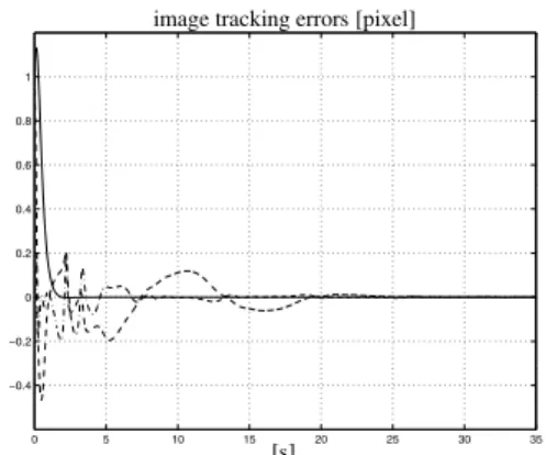
The system behavior is presented in Figures 3–8. The asymp-totic convergence of image tracking errors (planar and depth) can be observed in Figure 3.
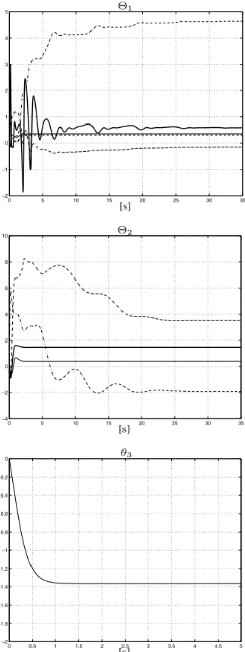
The parameters behavior is illustrated in Figure 4, where it can be observed that the parameters tend to a steady state
0 5 10 15 20 25 30 35
−0.4 −0.2 0 0.2 0.4 0.6 0.8 1
image tracking errors [pixel]
[s]
Figure 3: Image tracking errors:ec1(-·-); ec2(- -); es(-).
value after a adaptation period. The cartesian control signals can be considered adequate and they are depicted in Figure 5. The depth variation due to the tracking control is illustrated in Figure 6. The tracking of trajectory in the image frame is illustrated in Figure 7. Note that the tracking is well behaved despite the presence of input disturbances introduced by the depth control. Figure 8 shows the end-effector behavior in the 3D environment.
6
EXPERIMENTAL RESULTS
In this section, we present experimental results obtained by the implementation of the adaptive visual tracking controller proposed in Sections 3 and 4.
6.1
Workspace
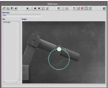
The experiments are performed on a 6DOF Zebra Zero ma-nipulator (IMI Inc.). A KPD-50 CCD camera (Hitachi Ltd.), with a lens of focal length f = 6.0 [mm], is mounted in front of the robot (see Figure 9 for a camera point of view). The extracted visual features are the image coordinates of a white sphere centroid located at the robot wrist and its im-age projected surface. The imim-ages of640×480[pixel] are acquired using a Meteor frame-grabber (Matrox Ltd.) at30 frames per second (FPS) with 256 grey levels. The image processing is performed on a50×50[pixel] sub-window, in order to guarantee that the sphere remains within the sub-window. The first estimations of the white sphere coordinates and area are performed off-line using a Graphical User In-terface (Figure 9), named VServo, developed in Tcl/Tk lan-guage. During task execution, features (centroid and area) are computed using the image moments algorithm (Haralick and Shapiro, 1993).
0 5 10 15 20 25 30 35 −2
−1 0 1 2 3 4
5 Θ1
[s]
0 5 10 15 20 25 30 35
−4 −2 0 2 4 6 8
10 Θ2
[s]
0 0.5 1 1.5 2 2.5 3 3.5 4 4.5 5 −2
−1.8 −1.6 −1.4 −1.2 −1 −0.8 −0.6 −0.4 −0.2
0 θ3
[s]
Figure 4: Adaptive parameters:Θ1,Θ2andθ3.
The joint velocity command generated by the adaptive con-trol law feeds the Zebra Zero (ISA board) which closes the velocity loop using an HCTL1100 microcontroller (HP Inc.) working in proportional velocity mode at0.52[ms].
Due to noise sensitivity, the proportional gain in the velocity loop is not high enough to eliminate steady state error due to gravity effect. This disturbance is identified off-line (using a least square method) and effectively compensated.
0 5 10 15 20 25 30 35
−5 −4 −3 −2 −1 0 1 2 3
[s] cartesian control [mm/s]
Figure 5: Control signals:v1(-·-); v2(- -);v3(-).
0 0.5 1 1.5 2 2.5 3 3.5 4 4.5 5 0.5
0.6 0.7 0.8 0.9 1 1.1
[s] depth [m]
Figure 6: Depth behavior.
−1 −0.8 −0.6 −0.4 −0.2 0 0.2 0.4 0.6 0.8 1 −1
−0.8 −0.6 −0.4 −0.2 0 0.2 0.4 0.6 0.8 1
image frame [pixel]
Xc1
X
c
2
Figure 7: Trajectories:xcM(-·-); xc(-).
6.2
Analysis of Results
0.5 0.6
0.7 0.8
0.9 1
−4 −3 −2 −1 0 1 −3 −2 −1 0 1 2
robot frame [mm]
X
Y
Z
Figure 8: End-effector trajectory.
Figure 9: Experimental setup.
[pixel/mm]. The initial conditions for the adaptive param-eters are θ3(0) = 0; Θ1(0) = [0 0 0 0 0]T; Θ2(0) =
[0 0 0 0]T. The control parameters are γ
3 = 5×10⁻³,
λm = 1.0, γ = 2×10⁻³ and λM = 1.0 respectively.
Other parameters are: Sc0= 860[pixel] forZ0= 1.0[m]
andS∗
c= 700[pixel].
Figure 10 shows the tracking errorsecandes. It can be
ob-served thatecandestends to small residual regions of orders
4[pixel] and10[pixel] respectively. Figure 11 presents the time history of the centroid position and the projected sur-face in the image frame. The cartesian control signal and the joint control signal are depicted in Figure 12. The tracking of trajectory in the image frame and the end-effector trajectory described in the workspace are shown in Figures 13 and 14 respectively.
0 20 40 60 80 100 120 140 160
−15 −10 −5 0 5 10
0 20 40 60 80 100 120 140 160
−50 0 50 100 150
[s]
planar tracking error [pixel]
depth tracking error [pixel]
Figure 10: Image errors:ec1(-·-); ec2(- -); es(-).
0 20 40 60 80 100 120 140 160
150 200 250 300 350 400
0 20 40 60 80 100 120 140 160
650 700 750 800 850 900
[s] centroid position [pixel]
projected surface [pixel]
Figure 11: xc1(-·-) ,xcd1(- -) , ; xc2(·) , xcd2(-); Sd(-) ,
Sc(- -).
0 20 40 60 80 100 120 140 160
−20 −10 0 10 20 30 40
0 20 40 60 80 100 120 140 160
−0.5 0 0.5 1
[s] cartesian control [mm/s]
joints control [rad/s]
Figure 12: Control signals : v1(-·-) ,v2(–) ,v3(- -); u1(-·-)
,u2(–) ,u3(- -).
220 240 260 280 300 320 340 360 −320
−300 −280 −260 −240 −220 −200
−180 image frame [pixel]
X
c
2
Xc1
Figure 13: Trajectories:xcM(-·-); xc(-).
0 20
40 60
80
200 250 300 350 400
40 60 80 100 120 140 160 180 200
robot frame [mm]
X
Y
Z
Figure 14: End-effector trajectory.
vary in an unknown pattern even in a well-conditioned envi-ronment. In order to overcome this drawback a filtering stage is used to reduce the noise in the area estimate.
7
CONCLUSION
In this paper, we have developed an adaptive visual servoing scheme, using an uncalibrated camera, that provides stable 3D cartesian tracking for robot manipulators without requir-ing depth measurement. The controller was designed to in-clude the general case of robotic systems in which all the im-age features were extracted from a spherical object. For the 1D depth subsystem, the MRAC control method was applied, whereas for the multivariable 2D tracking subsystem, the recently proposedSDU factorization method was adopted. Since a linearly parameterized model was obtained, no ex-plicit inverseimage Jacobianestimation was required in the control structure. The stability analysis for the proposed strategy was also presented with global properties. Simu-lation and experimental results with a real robot manipulator were included to illustrate the performance of the proposed strategy.
Future research topics following the ideas developed here are: navigation of autonomous vehicles using visual servo-ing, extension to full dynamics robots and application to hy-brid vision-force robot control.
REFERENCES
Conticelli, A. and Allotta, B. (2001a). Discrete-time robot vi-sual servoing in 3-d positioning tasks with depth adap-tation, ASME Journal of Dynamic Systems, Measure-ment and Control06(3): 356–363.
Conticelli, A. and Allotta, B. (2001b). Nonlinear controlabil-ity and stabilcontrolabil-ity analysis of adaptive image-based sys-tems,IEEE Transactions on Robotics and Automation
17(2): 208–214.
Corke, P. and Hutchinson, S. (2000). A new hybrid image-based visual servo control scheme,IEEE Conference on Decision and Control, pp. 2521–2527.
Costa, R. R., Hsu, L., Imai, A. and Kokotovic, P. (2003). Lyapunov-based adaptive control of MIMO systems,
Automatica39(7): 1251–1257.
Espiau, B., Chaumette, F. and Rives, P. (1992). A new ap-proach to visual servoing in robotics, IEEE Transac-tions on Robotics and Automation8(3): 313–326. Fang, Y., Behal, A., Dixon, W. E. and Dawson, D. M. (2002).
Adaptive 2.5d visual servoing of kinematically redun-dant robot manipulators,IEEE Conference on Decision and Control, Las Vegas, Nevada, pp. 2860–2865. Flandin, G., Chaumette, F. and Marchand, E. (2000).
Eye-in-hand/eye-to-hand cooperation for visual servoing,
IEEE International Conference on Robotics & Automa-tion, San Francisco, CA, pp. 2741–2746.
Haralick, R. M. and Shapiro, L. G. (1993). Computer and Robot Vision, Vol. II, Addison-Wesley.
Hsu, L. and Costa, R. R. (1999). MIMO direct adaptive control with reduced prior knowledge of the high fre-quency gain,IEEE Conference on Decision and Con-trol, Phoenix, Arizona, pp. 3303–3308.
Hsu, L., Zachi, A. R. L. and Lizarralde, F. (2001). Adaptive visual tracking for motions on smooth surfaces,IEEE Conference on Decision and Control, Orlando, Florida, pp. 1866–1871.
Hutchinson, S., Hager, G. and Corke, P. (1996). A tutorial on visual servo control,IEEE Transactions on Robotics and Automation12(5): 651–670.
Kelly, R., Carelli, R., Nasisi, O., Kuchen, B. and Reyes, F. (2000). Stable visual servoing of camera-in-hand robotic systems, ASME Journal of Dynamic Systems, Measurement and Control15(1): 39–48.
Malis, E., Chaumette, F. and Boudet, S. (1999). 2 1/2D visual servoing,IEEE Transactions on Robotics and Automa-tion15(2): 238–250.
Ortega, R., Hsu, L. and Astolfi, A. (2003). Immersion and invariance adaptive control of linear multivariable sys-tems,Systems and Control Letters49: 37–47.