Stability in a Class of Quartessence Models
A. M. Vel´asquez-Toribio
Federal University of Rio de Janeiro (UFRJ), Institute of Physics, P. O. Box 68528, CEP 21941-972, Rio de Janeiro, Brazil
Received on 13 April, 2006
Quartessence cosmological models with exponential and logarithmic equation of state are investigated using dynamical systems methods. We focus our analysis on the stability of these models.
Keywords: Cosmology; Quartessence; Dynamical systems; Stability
Progress in observational cosmology in the past few years suggests that the universe is dominated by two unknown com-ponents, namely, dark matter and dark energy. These two components have properties that are quite different from all the ordinary matter we know do exist in the physical world. Dark matter is a pressureless component, very important for structure formation, while dark energy, a negative pressure component, is responsible for the cosmic acceleration. From the point of view of simplicity, it would be interesting to de-scribe both components with a single equation of state (EOS). This idea is the main motivation for quartessence models that try to unify dark matter and dark energy in a single component [1]. The most studied quartessence model is the Chaplygin gas model [2], [3]. Nevertheless other EOS for quartessence exist as, for instance, those suggested in the work by Reis et al. [4].
In this work, we employ the methods of qualitative theory of dynamical system [5], [6] to study quartessence models with exponential and logarithmic EOS. Recently, M. Szyd-lowski and W. Czaja [7] investigated the structural stability of FRW cosmology with generalized Chaplygin gas. Here, we extend their analysis to other quartessence cosmologies.
This paper is organized as follows. In Section II, we briefly describe the dynamical systems techniques we use to analyze quartessence cosmological models. In Section III we analyze the critical points of the considered quartessence models. In Section IV we investigate the stability of the system using the Lyapunov’s method. Finally, in Section V we discuss the re-sults.
I. STUDY OF QUARTESSENCE MODELS WITH DYNAMICAL SYSTEMS
The main goal of quartessence cosmological models is to describe with a single equation of state, dark matter and dark energy. The prototype quartessence model is the generalized Chaplygin Gas (GCG) [3]. It is easy to show that for very high redshift these models behave like pressureless dark matter, while in the opposite limit the models asymptotically tend to a cosmological constant. Different aspects of the GCG models have been analyzed in the literature [2], [8], [9]. Recently, Reis et al. [4] suggested two other equations of state with the same asymptotic limits, namely Exponential and Logarithmic Quartessence [10]. It is clear that, in principle, many other equations of state can be used, but for the sake of
simplicity, and because they capture the main properties of this class of models, here we limit our analysis to these two cases. The considered models have the following EOS: Exponential Quartessence:
P=−M4e −ρα
M4 , (1)
Logarithmic Quartessence:
P=− M
4
h
ln(Mρ4)
iα, (2)
whereρis the density energy,Pthe pressure,Mhas dimension of mass andαis a dimensionless parameter.
We denote by H the Hubble parameter and the quanti-ties (H,ρ) are chosen as the phase space variables. We consider a homogeneous and isotropic Friedmann-Robertson-Walker(FRW) metric and we define our two-dimensional dy-namical system with the following equations:
˙
H=−H2−1
6(ρ+3P), (3)
˙
ρ=−3H(ρ+P), (4) where the dot denotes time derivative. We split in two parts, our discussion of the character of the critical points:
A) static case (H=0) and
B) non-static case (H6=0).
We consider non-degenerate critical points where the be-havior of the system in the neighborhood of the critical point is qualitatively equivalent to the behavior of its linear part. The linearization matrix of the system at the critical point(Ho,ρo)
is:
A=
Ã
−2H −1 6
d
dρ(ρ+3p) −3(ρ+p) −3Hddρ(ρ+p)
!
(H0,ρo)
As usual, the characteristic equation isdet(A−λI) =0, whereI is the identity matrix. The trace and the determinant for static critical points are [7],
TrA = 0 (5)
detA = −1
2(ρ+P) d
For non-static critical points we obtain:
TrA = −H(2+3 d
dρ(ρ+P))|(H0,ρo) (7)
detA = 6H2 d
dρ(ρ+P)|(H0,ρo) (8)
Here|(H0,ρo) denotes the value of the equation at the critical
point.
Since we are working with a two-dimensional dynamical system, the stability of the solution can be analyzed based on the sign of the trace and the discriminant [12]:
1. IfdetA<0, then the eigenvalues are real, have opposite signs and the critical point is a saddle point.
2. IfdetA>0 and the discriminant: D= (TrA)2−4detA> 0, then the eigenvalues are real, have the same sign and the critical point is a node. IfTrA>0 the critical point is an unstable point(node). IfTrA<0 the critical point is stable. 3. IfdetA>0 and the discriminant:D= (TrA)2−4detA<0, then the eigenvalues are complex conjugates and the critical point is a focus. IfTrA>0 the critical point is an unstable focus. IfTrA<0 it is a stable focus. In the case in which the eigenvalues are purely imaginary, the critical point is a stable neutral center.
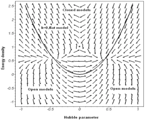
FIG. 1: The vector field portrait corresponding to the exponential quartessence case. For the figure we usedα=M4=1
II. TWO QUARTESSENCE MODELS
The two cosmological models that we are interested in have the property that their equation of statew=ρp is convex, i.e.
d2p
dρ2 <0. In this case, the maximum value of the sound speed
(c2s = d pdρ)is reached at the minimum value of the density. Some of the properties of these models have been discussed in [10]. In this section we consider the stability with the methods of qualitative analysis described in Section II.
A. Exponential Quartessence
For quartessence models, at early times, whenρ is large, we needw≈0, therefore, from Eq. (1), the parameterαcan not be negative. The minimal energy density of this model is given by ρmin=M4(W(α)
α ), whereW(x) is the Lambert
function defined to be the multi-valued inverse of the function W →WeW [10, 11]. Thus, whenρ=ρmin, the equation of
state parameter assumes the valuew=−1 (cosmological con-stant). The standardΛCDMis recovered when we substitute
α=0 in Eq. (1).
In the considered model the singular static point is given by:
Ho=0, ρo=M4
W(3α)
α (9)
After substituting Eqs. (1) and (9) into (6), we obtain:
detA=−1 2 (
M4
α W(3α)−M
4e−W(3α))(1+3αe−W(3α)) (10)
As the TrA=0, then, ifdetA>0, then the eigenvalues of the critical points have complex values, that correspond to the stable neutrally center type. Otherwise, as discussed above, if the determinant is negative the critical point represent a saddle point.
Let us now analyze the non-static critical points: H6=0. Equaling equations (3) and (4) to zero, we determine the non-static critical points :
ρo=
M4
α W(α), H
2
o=−
1 6(
M4
α W(α)−3M
4e−W(α)),
(11) Using Eqs. (7) and (8), we also obtain:
detA=6Ho2(1+αe−W(α)) (12) and
TrA=−Ho(2+3(1−αe−W(α))) (13)
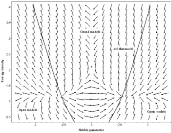
FIG. 2: The vector field portrait corresponding to the logarithmic quartessence case. For the figure we usedα=0.5,M4=1.
FIG. 3: The vector field portrait corresponding to the FRW model with cosmological constant.
FIG. 4: The vector field portrait corresponding to the FRW model with Chaplygin gas. For the figure we usedα=M4=1.
B. Logarithmic Quartessence
The logarithmic quartessence model EOS is given by equa-tion (2). In the following we consider only the non-static case. The minimum energy density is given byρmin=M4eαW(α
−1)
and the adiabatic sound speed isc2smax=1/W(α−1). Note that againΛCDMis recovered if we substituteα=0 in equation (2) [10]. Equalizing to zero Eqs. (3) and (4) and by using the equation of state (2) we obtain the following critical point (non-static case):
ρo=M4eαW(α
−1)
, Ho2=−M41 6[e
αW(α−1)
−3(αW(α−1)α]
(14) The value of the trace and the determinant are:
detA=6H02{1+ αM 4
(αW(α−1)α+1e
−αW(α−1)
} (15)
TrA=−H0{2+3(1+
αM4
αW(α−1)1+αe
−αW(α−1)
} (16) Similarly , as we did in the exponential case, we deduce from equation (15) that the determinant is always positive and, from the Eq. (16) the trace is negative for an expanding uni-verse(H>0). Therefore, the critical points (14) behave like an asymptotically stable node ifD>0 or as an asymptotically stable focus ifD<0. In Figure 2 we show the phase portrait in the logarithmic quartessence case.
In Figures 3 and 4 we show the phase portrait of the FRW models with a cosmological constant (positive) and Chaply-gin gas respectively, let us note the equivalence of the phase portraits in the physical domains(ρ≥0)of the four cosmo-logical models (Figs. 1, 2, 3 and 4) i.e. the structure of the phase space does not depend of the form of EOS. The behav-ior for the phase portraits are due to the fact that the stability of the critical point depends on the energy condition as discussed in [7].
III. LYAPUNOV FUNCTION AND QUARTESSENCE
There are different approaches to investigate the stability of dynamical systems. In the following we shall consider the Lyapunov function method.
The existence of a Lyapunov function,F, guarantees the stability of the dynamical system aroundx0. Furthermore, if the inequalitydFdt ≤0 holds in a neighborhoodUx0, thenx0is
asymptotically stable. For a mathematical discussion of this method see e.g. refs. [13–15].
For the two-dimensional dynamical system (3) and (4) we propose the following Lyapunov’s function:
F(ρ,H) =ρ+H 2
2 >0 (17)
The above function is positive definite ifρ>0. From equa-tions (3)-(4) we have critical points ifH=0 andw=−1
H2=ρ3 withw=−1, and they represent asymptotic sates of the universe.
We also assume an expanding Universe and, in order to as-sure the asymptotic stability of the system of equations, we require thatFfirst total derivative be negative. Therefore, we can write:
dF dt =
dρ
dt +H dH
dt ≤0 (18)
In an expanding universe (H>0) withw≥ −1 the energy density obeys the conditionddtρ≤0. Using Eq. (3) the quantity
dH
dt can be cast in the following form
dH dt =−[
ρ
3− k a2+
(ρ+3P)
6 ] (19)
On the other hand, if we now use the definitions of the density parameters: Ωk=−k/a2H2,ΩQ=ρ/3H2and since Ωk+ΩQ=1, it is easy to show that:
dH dt =−
ρ
3[ 3
2(1+w) +
(1−ΩQ)
ΩQ ] (20)
From Eqs. (20) and (4) we have,
dF dt =−(
7
2(1+w)Hρ+Hρ
(1−ΩQ)
ΩQ
) (21)
ΩQ≥ −
2
7w+5 (22)
The last equation is the condition for stability of the dynam-ical system (3)-(4) with quartessence EOS in the casew≥ −1. The important point here is the existence of the Lyapunov function satisfying condition (22). In summary, the function F has a minimum (when ΩQ= 7ω+−25) on the critical point
and there is a neighborhood (the attraction basin) withH>0 where F has non-positive time derivative. Hence, this asymp-totic states of the universe are asympasymp-totically stable.
IV. CONCLUSIONS
In the present paper we consider the stability of two quartessence models, one with an exponential EOS and the other with a logarithmic one. The dynamics is studied in the phase plane(H,ρ) at a finite domain, applying methods of the qualitative theory of dynamical systems. We considered hyperbolic critical points. For both, the exponential and log-arithmic cases, if the Hubble function is positive the models are stable in the neighborhood of the critical points. There-fore, it is interesting that the requirement of stability for these quartessence models yields an Universe which accelerates, in accordance with observational evidences at present [17].
To study the asymptotic behavior of the above mentioned quartessence cosmological models we have applied the Lya-punov method. We have shown that exists a LiaLya-punov func-tion (F) given by Eq.(17). This function can be thought as a generalized energy function for the system, and it leads us to the stability condition given by Eq.(22).
In summary, in this work we showed that quartessence models with exponential and logarithmic EOS are stable in their physical domains. Therefore, since the real world is also dynamically stable [13], these quartessence models, from the theoretical point of view, in principle, might describe the late-time acceleration of the Universe. Finally we remark that, for adiabatic perturbations, the matter power spectrum for these quartessence models present instabilities and oscil-lations [18]. However, as shown in [10], this kind of problem can be solved by considering a special type of non-adiabatic perturbation.We believe that these quartessence models de-serve to be further investigated.
V. ACKNOWLEDGMENTS
The author wish to thank Ioav Waga for several useful dis-cussions that helped us to improve this work and the Brazilian research agency for financial support: CNPq.
[1] M. Makler, S. Q. Oliveira, and I. Waga, Phys. Lett. B555, 1 (2003).
[2] A. Kamenshchik, U. Moschella, and V. Pasquier, Phys. Lett. B 511,265 (2001) ; N. Bilic, G. B. Tupper, R. D. Viollier, Phys. Lett. B535, 17 (2002).
[3] M. C. Bento, O. Bertolami, and A. A. Sen, Phys. Rev. D66, 043507 (2002).
[4] R. R. R. Reis, M. Makler, and I. Waga, Phys. Rev. D69, 101301 (2004).
[5] O. I. Bogoyavlensky, Methods in Qualitative Theory of Dynam-ical Systems in Astrophysics and Gas Dynamic (Springer - Ver-lag, Berlin 1985).
[6] J. Wainwright and G. F. R. Ellis, Dynamical System in Cosmol-ogy, Cambridge University Press (1997).
[7] M. Szydlowski, W. Czaja, Phys. Rev. D69, 023506 (2004). [8] M. Makler, S. Q. Oliveira, and I. Waga, Phys. Rev. D 64,
123521 (2003).
[9] P. P. Avelino, L. M. G. Beca, J. P. M. de Carvalho, C. J. A. P. Martins, and P. Pinto, Phys. Rev. D67, 023511 (2003). [10] R. R. R. Reis, M. Makler, and I. Waga, Class. Quantum. Grav
22, 353 (2005).
[11] S. R. Cranmer, American J. Phys.,72, 1397 (2004).
[12] D. V. Anosov and V. I. Arnold, Dynamical Systems I, Ency-clopaedia of Mathematical Sciences, Volume 1 (1980). [13] L. H. A. Monteiro,Sistemas Dinamicos, Editora Livraria da
Fisica (2002).
[15] T. C. Charters, A. Nunes, and J. P. Mimoso, Class. Quant. Grav. 18, 1703 (2001).
[16] D. J. Albers, J. C. Sprott, DOI: SFI-WP 04-02-007, SFI Work-ing Papers (2003).
[17] S. Perlmutteret al., Nature319, 51 (1998); S. Perlmutteret al.,
Astrophy. J.517, 565 (1999); A. G. Riesset al., Astrom. J.116, 1009 (1998).