Multi-satellite sensor study on precipitation-induced emission pulses of NO<sub><i>x</i></sub> from soils in semi-arid ecosystems

(1)

www.atmos-chem-phys.net/16/9457/2016/ doi:10.5194/acp-16-9457-2016

Multi-satellite sensor study on precipitation-induced emission pulses

of NO

x

from soils in semi-arid ecosystems

Jan Zörner1, Marloes Penning de Vries1, Steffen Beirle1, Holger Sihler1,3, Patrick R. Veres2,a, Jonathan Williams2, and Thomas Wagner1

1_{Satellite Remote Sensing Group, Max Planck Institute for Chemistry, Mainz, Germany} 2_{Atmospheric Chemistry Department, Max Planck Institute for Chemistry, Mainz, Germany} 3_{Institute of Environmental Physics, University of Heidelberg, Heidelberg, Germany} a_{now at: NOAA Earth System Research Laboratory, Boulder, CO, USA}

Correspondence to:Jan Zörner ([email protected])

Received: 29 January 2016 – Published in Atmos. Chem. Phys. Discuss.: 25 February 2016 Revised: 27 June 2016 – Accepted: 10 July 2016 – Published: 29 July 2016

Abstract.We present a top-down approach to infer and quan-tify rain-induced emission pulses of NOx (≡NO+NO2), stemming from biotic emissions of NO from soils, from satellite-borne measurements of NO2. This is achieved by synchronizing time series at single grid pixels according to the first day of rain after a dry spell of prescribed duration. The full track of the temporal evolution several weeks before and after a rain pulse is retained with daily resolution. These are needed for a sophisticated background correction, which accounts for seasonal variations in the time series and allows for improved quantification of rain-induced soil emissions. The method is applied globally and provides constraints on pulsed soil emissions of NOxin regions where the NOx bud-get is seasonally dominated by soil emissions.

We find strong peaks of enhanced NO2 vertical column densities (VCDs) induced by the first intense precipitation after prolonged droughts in many semi-arid regions of the world, in particular in the Sahel. Detailed investigations show that the rain-induced NO2pulse detected by the OMI (Ozone Monitoring Instrument), GOME-2 and SCIAMACHY satel-lite instruments could not be explained by other sources, such as biomass burning or lightning, or by retrieval artefacts (e.g. due to clouds).

For the Sahel region, absolute enhancements of the NO2 VCDs on the first day of rain based on OMI measurements 2007–2010 are on average 4×1014molec cm−2_{and exceed} 1×1015molec cm−2 _{for individual grid cells. Assuming a} NOx lifetime of 4 h, this corresponds to soil NOx emis-sions in the range of 6 up to 65 ng N m−2_s−1_{, which is}

in good agreement with literature values. Apart from the clear first-day peak, NO2 VCDs are moderately enhanced (2×1014molec cm−2_{) compared to the background over the} following 2 weeks, suggesting potential further emissions during that period of about 3.3 ng N m−2_s−1_{. The pulsed} emissions contribute about 21–44 % to total soil NOx emis-sions over the Sahel.

1 Introduction

(2)

night, N2O5hydrolysis on aerosol surfaces is the dominant sink of NOx(Jacob, 1999).

While anthropogenic activity such as fossil-fuel combus-tion is the largest source of NOx, there are also important natural sources including natural biomass burning from for-est fires, lightning and microbial processes in soils. Soil emissions of NOx (sNOx) constitute an estimated fraction of ≈15 % of total NO_x on a global basis (Warneck and

Williams, 2012; Hudman et al., 2012) and may even dom-inate the local NOxbudget in non-industrialized regions like remote tropical and agricultural areas (Yienger and Levy, 1995; Steinkamp et al., 2009). Bottom-up approaches using global chemistry models suggest global fluxes between 4 and 15 Tg N yr−1_{with uncertainties of up to 5–10 Tg N yr}−1_(e.g. Yienger and Levy, 1995; Steinkamp and Lawrence, 2011; Hudman et al., 2012; Vinken et al., 2014, and references therein). Satellite constrained top-down approaches hint at regional underestimations of sNOxof a factor of 2 and more (Jaeglé et al., 2004; Wang et al., 2007; Boersma et al., 2008; Zhao and Wang, 2009; Vinken et al., 2014). Thus, global emissions of sNOxremain uncertain.

Emissions of NOxfrom natural and anthropogenically in-fluenced soils are mainly driven by microbial activity within the top soil layer and associated chemical reactions (Conrad, 1996). Primarily, two important groups of micro-organisms, nitrifiers and denitrifiers, are involved in processes related to the turnover of nutrients in the soil (Pilegaard, 2013; Behrendt et al., 2014). They are directly responsible for the corresponding processes of (i) nitrification, the biological ox-idation of nitrogen compounds, typically the oxox-idation of soil ammonium (NH+

4) to nitrate (NO

−

3) and (ii) denitrification, the reduction of nitrate by microbes to gaseous products, i.e. N2O and finally N2. NO is a gaseous by-product of both processes and once released reacts with ambient O3, to form NO2 and oxygen (O2) within minutes. Findings from Os-wald et al. (2013) suggest that gaseous nitrous acid (HONO), which is rapidly photolysed to NO, is also emitted from soils. Most soil emissions of NO in semi-arid areas are linked to microbial processes, but some chemical (abiotic) forma-tion processes of NO are known to exist, which are more important for acidic soils with high nitrite (NO−

2) concen-trations (Davidson, 1992b). Such soils are found in humid regions, i.e. the humid tropical belt and the northern tem-perate zone, where soil leaching removes alkaline material and associated salts from the soil profiles leading to pH val-ues of less than 5.5 (Merry, 2009). Emissions of nitrogen-containing gases, such as NO, N2and N2O increase dramat-ically in soils with enhanced nitrogen availability due to the presence of N-fixing microbial species and plants (Virginia et al., 1982; van Groenigen et al., 2015). In semi-arid areas with sparse vegetation cover, surfaces are covered by a vari-ety of communities of cyanobacteria, algae, lichens, mosses, microfungi, and other bacteria in differing proportions (Bel-nap and Lange, 2001; Barger et al., 2005). Associated organ-isms within these biological crusted soils fix atmospheric N2

and, thus, raise the nitrogen availability in the soil (Evans and Ehleringer, 1993). Barger et al. (2005) found varying rates of soil NO fluxes from biologically crusted soils that differed in their nitrogen fixation potentials. Recent findings from We-ber et al. (2015) suggest that dryland emissions of reactive nitrogen are largely driven by biocrusts rather than the un-derlying soil and strongly depend on the soil water content (SWC), i.e. precipitation events. Throughout this study, for simplicity all emissions from soils and biocrusts are referred to as sNOx.

Soil emissions of trace gases depend on a wide range of ambient environmental conditions such as soil type, soil moisture, temperature, pH-Value and nitrogen content (Con-rad, 1996; Ludwig et al., 2001; Meixner and Yang, 2006; Oswald et al., 2013). Also agricultural management prac-tices, such as soil cultivation, fertilization and irrigation can strongly affect the fluxes (Bouwman et al., 2002). In remote regions like the Sahel, where synthetic fertilizer is limited, manure plays a prominent role in the fertilization of agricul-tural fields and can contribute significantly to the input of or-ganic nitrogen into the soil (Schlecht and Hiernaux, 2004; Delon et al., 2010). The effective NOx fluxes from soils to the atmosphere are potentially offset by “canopy reduc-tion” where nitrogen oxides are quickly deposited on avail-able vegetation surfaces (Ganzeveld et al., 2002). During the dry season in tropical ecosystems soils accumulate in-organic nitrogen through N-fixing micro-organisms. Subse-quently, water-stressed microbes trapped in the soil become activated by the first rain event of the wet season and release NO as a by-product of nitrogen consumption (Davidson, 1992a). Rain-induced pulsing events of NOxemissions were observed in situ and by laboratory measurements of soil sam-ples (e.g. Williams et al., 1987, 1992; Johansson and San-hueza, 1988; Levine et al., 1996; Scholes et al., 1997; Kim et al., 2012; Wang et al., 2015). Pulsed emissions of sNOx occurring at the transition phase between the dry and wet season, were previously also observed from space (Jaeglé et al., 2004; Bertram et al., 2005; Hudman et al., 2012) in the Sahel region. Hudman et al. (2012) showed that intense but short events of soil emissions, i.e. pulsed emissions, at the start of the wet season after a prolonged dry spell represent a large fraction of annual soil emissions in the Sahel region. As noted by Hudman et al. (2012) further research needs to be done to verify that the observed pulses by OMI (Ozone Monitoring Instrument) are not biased by the retrieval algo-rithm.

(3)

We introduce an optimized algorithm that synchronizes and averages multiple time series of atmospheric variables either from one location only, or from individual grid pixels, by aligning them on a relative timescale to each other. Our algorithm enhances the basic approach described by Hud-man et al. (2012) with several features: (i) performing the analysis globally with (ii) high spatial resolution, which is both achieved by expanding the time span of the study to several years (2007 to 2010) enabling an investigation of sin-gle grid pixels of 0.25◦ _{with reasonable statistics. (iii) The}

full track of the temporal evolution several weeks before and after a rain pulse is retained with daily resolution. (iv) By in-tercomparing measurements of NO2from multiple satellite instruments it is possible to quantify potential measurement artefacts and investigate the impact of different retrieval al-gorithms. Furthermore, sensitivity studies are conducted in order to evaluate the impact of the a priori assumptions on thresholds for daily rainfall, i.e. the definition of drought, and its requested duration.

Our approach is a purely top-down method, in the sense that satellite data of trace gases are exclusively used to de-scribe and quantify phenomena taking place on the Earth’s surface and atmosphere. It is, therefore, extremely important to consider natural processes in the atmosphere that could trigger soil emissions or may affect the retrieved NO2 col-umn densities in other ways. In order to achieve this we in-corporate total columns of water vapour, humidity, temper-ature and wind directions in our analysis to assess the pre-vailing meteorology. To verify that the observed responses in the trace gas column densities reflect the impact of emis-sion fluxes from the soil, possible interferences from other parameters, e.g. fires, modified cloud fractions, coincidences with lightning events and horizontal transport from polluted regions, are also investigated.

Veres et al. (2014) found in laboratory experiments that also several VOCs including HCHO exhibit pulsed emissions when dry soils are first wetted. Our study, hence, also ad-dresses the question whether HCHO emissions from semi-arid soils can be observed from satellite-borne sensors.

In contrast to previous satellite studies, our study makes a clear distinction between (i) pulsed emissions, which show strong gradients on a day-to-day scale triggered by a singular precipitation event and (ii) background emissions, which are not directly affected or could not be unambiguously related to a strong precipitation pulse. This facilitates the assessment of the contribution from single sNOx pulses additionally to background levels.

The paper is organized as follows: in Sect. 2, all data prod-ucts used within this study are presented. In Sect. 3, the basic algorithm used for averaging the time series of environmental parameters along a relative time axis around the first day of precipitation is described. In Sect. 4, this approach is then ap-plied to areas with different spatial extents. We first perform an analysis on a global scale to delineate regions that show pronounced features in sNOxin response to the first rain after

a prolonged dry spell. In a second step, we focus on Africa and the Sahel region, in specific, and separate the analysis for different seasons. For this region, we investigate fundamen-tal relationships between soil emissions and some of their governing parameters, i.e. soil moisture content, tempera-ture, air humidity. Within this analysis possible interferences from other parameters are also investigated, and detailed sen-sitivity studies are conducted. In Sect. 5, sNOxemissions are inferred from the NO2VCDs based on a sophisticated back-ground correction. A list of acronyms for commonly used instruments and products in this paper is provided in Table 1.

2 Data

2.1 Satellite observations of trace gases

Vertical column densities (VCDs) of NO2 and HCHO can be retrieved from nadir-viewing satellite instruments, by analysing solar backscatter radiances in the UV–VIS (ultraviolet–visible) spectral range. Differential Optical Ab-sorption Spectroscopy (DOAS; Platt and Stutz, 2008), which exploits characteristic narrow absorption structures, is typi-cally used for the analysis.

Tropospheric VCDs are usually derived in a multi-step process (e.g. Boersma et al., 2004, 2007; De Smedt et al., 2008, 2012). First, total slant column densities (SCDs) are re-trieved, i.e. the integrated concentrations along the effective light path, by fitting the measured spectrum with a model tak-ing into account all other absorbers in the atmosphere. Sec-ond, tropospheric SCDs are derived by subtracting the strato-spheric column (NO2) or a latitude-dependent bias estimated over the Pacific (HCHO). Third, the tropospheric SCDs are then translated to tropospheric VCDs. The conversion of SCDs to VCDs is usually performed by dividing the SCDs by a so-called air mass factor (AMF) (Solomon et al., 1987). The AMF is derived from radiative transfer simulations tak-ing into account information of ground albedo, aerosols and clouds, the vertical profile of the trace gas and the satellite viewing geometry (e.g. Palmer et al., 2001; Richter and Bur-rows, 2002; Martin, 2003).

(4)

Table 1.List of acronyms for commonly used instruments and products in this paper.

Abbreviation Name References

CMORPH CPC (Climate Prediction Center) MORPHing technique Joyce et al. (2004) DOMINO Derivation of OMI tropospheric NO2project (v2.0) Boersma et al. (2011) ECMWF European Centre for Medium-Range Weather Forecasts Dee et al. (2011) FRESCO+ Fast Retrieval Scheme for Clouds from the Oxygen A band Wang et al. (2008)

GOME Global Ozone Monitoring Experiment Burrows et al. (1999)

GOME-2 Global Ozone Monitoring Experiment-2 Callies et al. (2000); Munro et al. (2006, 2016)

MERIS MEdium Resolution Imaging Spectrometer Rast et al. (1999) MODIS Moderate Resolution Imaging Spectroradiometer Kaufman et al. (1998) OMCLDO2 Cloud Pressure and Fraction using O2-O2absorption Acarreta et al. (2004)

OMI Ozone Monitoring Instrument Levelt et al. (2000, 2006)

PERSIANN Precipitation Estimation from Remotely Sensed Information using Artificial Neural Networks

Sorooshian et al. (2000)

SCIAMACHY SCanning Imaging Absorption spectroMeter for Atmospheric CHartographY

Bovensmann et al. (1999)

SMMR Scanning Multi-channel Microwave Radiometer Gloersen and Barath (1977)

SSM/I Special Sensor Microwave Imager Wentz and Spencer (1998); Wentz

(2013)

TMI TRMM Microwave Imager Wentz et al. (2001)

TMPA Tropical Rainfall Measuring Mission Multisatellite Precipitation Analysis

Huffman et al. (2007)

TRMM Tropical Rainfall Measuring Mission Simpson et al. (1996); Huffman et al. (2007)

TROPOMI TROPOspheric Monitoring Instrument Veefkind et al. (2012)

WWLLN World Wide Lightning Location Network Dowden et al. (2002); Lay et al. (2004); Rodger et al. (2006)

without precipitation generally corresponds to a change in cloud cover, cloud effects need to be investigated. Therefore, satellite measurements retrieved under low and high cloud fractions are studied in detail using cloud information, de-rived from FRESCO+ (Wang et al., 2008) for GOME-2 and SCIAMACHY and OMCLDO2 (Acarreta et al., 2004) for OMI.

2.2 Satellite instruments and trace gas products

SCIAMACHY (Bovensmann et al., 1999) aboard the EN-VISAT satellite was operated from 2002 to 2012. It had a ground pixel size of about 30 km×60 km (VIS) to 30 km×120 km (UV). GOME-2 (Callies et al., 2000; Munro et al., 2006) aboard ESA’s METOP-A satellite, launched in 2007, has a ground pixel size of about 40 km×80 km. OMI (Levelt et al., 2000, 2006) on NASA’s Aura platform, which was launched in 2004 has a ground pixel size of 13 km×24 km at nadir and increasing pixel sizes to the far ends of the 2600 km wide swath. In our study, the two out-ermost pixels are screened out to remove the pixels with the largest viewing angles and lowest spatial resolution. The lo-cal overpass times for the three satellite instruments at the Equator are about 09:30 a.m. for GOME-2, 10:00 a.m. for SCIAMACHY and 01:30 p.m. LT for OMI.

For NO2, the products GOME-2 TM4-NO2A version 2.3, SCIAMACHY TM4-NO2A version 2.3 and OMI DOMINO version 2.0.1 are used (Boersma et al., 2004, 2011). For HCHO the products GOME-2 version 12, SCIAMACHY version 12 and OMI version 14 are used (De Smedt et al., 2012). Data products are provided freely by the Tropo-spheric Emission Monitoring Internet Service (TEMIS) via http://www.temis.nl/.

Differences among the trace gas data products from the three satellite instruments are expected due to, among oth-ers, the calculation of the AMF, their different ground pixel size, local overpass time, cloud products used, the diurnal cycle of cloud conditions and the covered time period. Fur-thermore, the diurnal cycle of the instantaneous NOx life-time and emissions might also cause systematic differences between SCIAMACHY and GOME-2 on the one hand, and OMI on the other.

Uncertainties of tropospheric NO2 VCDs result mainly from uncertainties of the stratospheric correction (about 2×

(5)

2.3 Precipitation

The estimation of precipitation on a daily global scale is facilitated through the combination of radar, passive mi-crowave, VIS and infrared (IR) sensors aboard low-Earth or-biting as well as geostationary satellites. In this study, three different products are used that employ such a blended pre-cipitation scheme. All three data sets agree in their spatial resolution (0.25◦_×_0.25◦_{) and provide data in 3-hourly time}

steps, i.e. 12:00 UTC covering the period 22:30 to 01:30 UTC and so on. They are briefly described below.

The Tropical Rainfall Measuring Mission (TRMM) Multi-satellite Precipitation Analysis (TMPA) 3B42 Version 7 data set (Huffman et al., 2007) combines observations made by the TRMM satellite with other satellite systems, as well as land surface precipitation gauge analyses when possible. The passive microwave data, which has a strong physical relation-ship to the hydrometeors that result in surface precipitation, are collected from the Microwave Imager (TMI) on TRMM, Special Sensor Microwave Imager (SSM/I) on Defense Me-teorological Satellite Program (DMSP) satellites, Advanced Microwave Scanning Radiometer – Earth Observing System (AMSR-E) on Aqua, and the Advanced Microwave Sound-ing Unit-B (AMSU-B) on the National Oceanic and Atmo-spheric Administration (NOAA) satellite series. The IR data, for the TMPA are collected by the international constellation of geosynchronous satellites. Additionally, data from TMI and the precipitation radar (PR) on TRMM are used as a source of calibration. The whole TMPA algorithm is con-structed in four steps: (i) microwave precipitation estimates are calibrated and merged. (ii) IR precipitation data are pro-duced using the calibrated microwave results. (iii) Then, the microwave and IR precipitation estimates are combined fill-ing missfill-ing data. (iv) Lastly, rain gauge data are incorporated for the final product. For a detailed explanation of the TMPA algorithm see Huffman et al. (2007).

A similar approach is used for the CMORPH product (CPC MORPHing technique; Joyce et al., 2004), which uses passive microwave information from SSM/I, AMSU-B, AMSR-E and TMI. The main difference to TMPA is that data gaps are treated differently by transporting rainfall features via spatial propagation information, which is obtained from geostationary satellite IR data (Joyce et al., 2004).

PERSIANN (Precipitation Estimation from Remotely Sensed Information using Artificial Neural Networks; Sorooshian et al., 2000) assimilates IR precipitation esti-mates from geosynchronous satellites. These estiesti-mates are then calibrated using microwave precipitation from low Earth orbit satellites. It differs from the other above-described pre-cipitation algorithms as its calibration technique involves an adaptive training algorithm that updates the retrieval param-eters when microwave observations of precipitation become available (Sorooshian et al., 2000).

Inter-comparison studies show good agreement with ground-based precipitation observations for these data

prod-ucts (e.g. Ebert et al., 2007; Novella and Thiaw, 2010; Romilly and Gebremichael, 2011; Liu et al., 2015; Pipunic et al., 2013; Pfeifroth et al., 2016, and references therein), which is, however, variable for different geographic regions, surface types and rain intensities.

In our study, we apply each precipitation product individ-ually to differentiate between days with or without rain fall. From the comparison of the corresponding results we find that the uncertainties and differences among the precipita-tion data sets have only minor effects on the obtained results (see Appendices A, E).

2.4 Soil moisture

The processes of nitrification and denitrification, which gov-ern sNOx fluxes, are closely related to the soil water con-tent (Meixner and Yang, 2006). In situ measurements of soil moisture are sparse and difficult to extrapolate to broad ge-ographic regions due to their highly heterogeneous nature. Combined satellite measurements of soil moisture overcome this issue by providing global coverage on a daily basis. Al-though the absolute value of soil moisture from merged satel-lite products has large uncertainties, relative variations trig-gered by precipitation events, should be evident in the time series.

Here, we use data from the ESA Soil Moisture CCI (Cli-mate Change Initiative) ECV project, which merges level 2 soil moisture data derived from multiple satellite sensor products (Wagner et al., 2012) in order to construct a con-sistent long-time data set. Among the list of sensors that are included, are the C-band scatterometers on board of the ERS and METOP satellites and the multi-frequency radiome-ters SMMR, SSM/I, TMI, AMSR-E, and Windsat. The data sources include active (scatterometer) and passive (radiome-ter) microwave observations acquired preferentially in the low-frequency microwave range.

2.5 Other data sets

The data sets described above provide the basic information used in our research study. To evaluate and understand other influences on the retrieved trace gas levels; however, further atmospheric and environmental parameters are considered.

2.5.1 Lightning NOx

(6)

(Dow-den et al., 2002). This algorithm is, thus, more sensitive to cloud-to-ground flashes because of their stronger radiation in the VLF band compared to intra-cloud flashes. In order to be classified as a lightning event the lightning strike must be detected by at least five stations. The detection efficiency (DE) varies to a large extent due to the spatial distribution of contributing stations. For example, over Australia the DE is

≈80–90 %, but only≈10–20 % over Africa (Rodger et al.,

2006).

2.5.2 Fire activity

Biomass burning in specific regions is a major source of trace gases and aerosol particles (Crutzen and Andreae, 1990) and, therefore, must be considered in our analysis. The MODIS global monthly fire location product MCD14ML (Giglio et al., 2006) is used to filter out locations affected by fires.

2.5.3 Meteorology

In order to understand the prevailing meteorology and fil-ter for special circumstances in the Sahel region, modelled data of soil and air temperature, pressure, humidity as well as wind fields are taken from the ECMWF ERA-Interim analy-sis (Dee et al., 2011). The model data are acquired at a spatial resolution of 0.25◦_{and a temporal resolution of 6 h over the}

period from 2007 to 2010. The data are publicly available via http://apps.ecmwf.int/datasets/.

2.5.4 Land cover

The analysis of trace gas time series is also split up for dif-ferent land cover types as they are related to difdif-ferent soil compositions and, thus, different sNOx potentials. Here, a land cover map for the year 2009 from the ESA initiated GlobCover project is used, which utilizes observations from the MERIS sensor on board the ENVISAT satellite mission with a spatial resolution of 300 m. The product is publicly available via http://due.esrin.esa.int/page_globcover.php and comprises 22 land cover classes defined with the United Na-tions (UN) Land Cover Classification System (LCCS) with an overall accuracy across all classes of 58 % (Arino et al., 2007; Bontemps et al., 2011). The data are downscaled using a most-common-value approach to identify dominant land cover types and to match the resolution of the other data sets. Thus, misclassifications might occur particularly over heterogeneous terrain and transition zones, while classifica-tion over homogeneous terrain is expected to be robust.

2.5.5 Water vapour

Total column observations of H2O VCDs from GOME-2 give insight into the absolute humidity of the atmosphere at the time of the NO2 observation from GOME-2 and, thus, a temporally more reliable estimate compared to modelled ECMWF data. H2O VCDs from GOME-2 are derived based

00 UTC 00 UTC

13:30 UTC 13:30 UTC

Current day Next day

Previous day

Accumulated precipitation (3–hourly products) Approximate satellite overpasses

Figure 1.Schematic of the 24 h time period selected for the inte-gration of precipitation data. The eight 3-hourly precipitation rates prior to the overpass times of the SCIAMACHY, GOME-2 and OMI satellite sensors are summed.

on a DOAS retrieval using a H2O absorption band around 650 nm. Remaining non-linearities due to saturation effects are accounted for by a simple correction function determined from a radiative transfer model (RTM). Empirical AMFs are derived from the simultaneously measured O2 absorption. Retrieval details and validation of the H2O VCDs can be found in Wagner et al. (2003, 2006) and Grossi et al. (2015).

3 Methodology

A daily global time series data set spanning from 2007 to 2010 for grid boxes of 0.25◦_×_0.25◦_{is established}

compris-ing total precipitation and trace gas measurements. Level 2 products of the trace gases are screened for observations with effective cloud fraction above 20 % and a solar zenith angle above 60◦

. Furthermore, observations coinciding with light-ning or fire events on the same day and within the same grid box are filtered out.

The 3-hourly precipitation data are integrated over the 24 h period prior to the satellite overpasses of GOME-2, SCIA-MACHY and OMI to collocate rainfall events and trace gas observations. For example, in the Sahel region, which is the main study region of this paper, the precipitation data are in-tegrated from 13:30 UTC of the previous day to 13:30 UTC of the current day as this corresponds to the local overpass time of OMI. This 24 h period is calledDayin the follow-ing pages (see Fig. 1). For the global analysis, the temporal integration is shifted by 3 h in steps of 45◦_longitude.

(7)

reason-5 4 3 2 1 0 1 2 3 4 reason-5 Days before and after first rainfall 0.0

0.2 0.4 0.6 0.8 1.0 1.2 1.4 1.6

OMI NO

2

VCDs [1e15 molec cm

-2]

5 4 3 2 1 0 1 2 3 4 5 Days before and after first rainfall 0

1 2 3 4 5 6 7

Precipitation [mm]

Threshold

Figure 2.Time series of TMPA precipitation(a)and OMI NO2VCDs(b)for a 10 day period around the first rain event for a single grid pixel in the Sahel on 11 April 2008 at 15.25◦_{N, 25.5}◦_{E. A threshold of 2 mm precipitation per day is chosen and at least 60 days of drought}

are required.

able amount of precipitation on the first rain day (>2 mm). Then, the trace gas column densities around thisfirst day of rainfall, which is counted asDay 0hereafter, are compared to the background levels during the preceding dry spell. The re-sults vary slightly for different thresholds of the precipitation trigger, as shown in Appendix C. These sensitivity tests also show that a threshold of 2 mm day−1_{leads to good statistics} as well as representative responses in NO2VCDs.

Figure 2 depicts a typical time series of precipitation (left panel) and NO2VCDs (right panel) for a 5-day period around the first rain event (on Day 0) after a dry spell for a sin-gle grid pixel in the Sahel in April 2008. In the following, the days around the first day of rainfall are referred to as Day−3, Day−2, Day−1, Day 0, Day+1, Day+2, Day+3 and so forth. It should be noted that there are almost no gaps in the precipitation time series; however, there are many in the trace gas time series. This is primarily due to the lower spatio-temporal coverage of trace gas products as well as the cloud, lightning and fire screening. In the example shown in Fig. 2 a 0.25◦_×_0.25◦_{pixel is chosen, which provides a}

complete NO2time series over 10 days. There is very little precipitation per day before the initial rain event. On Day 0, precipitation exceeds a threshold of 2 mm, used to differen-tiate between “rain” and “no rain”. Investigating the time se-ries of NO2around the first day of rainfall reveals a strong enhancement on Day 0 and some smaller enhancement on Day−1 and Day+1, whereas from Day−10 to Day−2 the NO2VCD is close to the pre-event level; i.e. the average NO2 VCDs of Day−5 to Day−1. NO2VCDs after Day+1 stay systematically higher than the background.

The time series for this single grid box represents the evo-lution of precipitation and trace gas VCDs around the first day of rainfall for a single grid pixel (experiencing first pre-cipitation after an extended drought) demonstrating the basic principle of this study.

In order to achieve representative results with improved statistics, averaging the time series over many pixels is nec-essary. However, as we focus on pulsed soil emissions,

av-eraging of time series from different pixels with rain events shifted in time has to be avoided. Furthermore, only a small subset of all possible pixels and their corresponding time se-ries fulfils the conditions of the precipitation trigger. Thus, the individual time series are first synchronized in time rela-tive to the first day of rainfall (Day 0). The subsequent aver-aging method is applied, in the following section, either with focus on high spatial resolution or with focus on best statis-tics at the expense of losing spatial resolution by averaging over larger areas.

In the following sections a drought period of at least 60 days followed by a rain event (precipitation>2 mm) is re-ferred to as the reference case. The drought period of about 2 months is chosen as we find the highest response in NO2with this setting. In Appendix B, the impact of drought lengths on the derived soil emission pulses is investigated.

4 Results

4.1 Global analysis

The algorithm described above, is applied to the full spatial extent covered by the TRMM/TMPA precipitation data set (−180 to 180◦_{longitude, 50 to}₋₅₀◦_latitude).

Figure 3a displays the number of valid OMI observations on 1.25◦_×_1.25◦_{grid pixels that fulfil the selection criteria,}

i.e. 60 days of drought and at least 2 mm of precipitation on Day 0. For most regions in the world enough data points are found for our analysis; exceptions are regions with no pronounced seasonality in rainfall (e.g. tropical rainforests, North America, Europe) and regions where rain occasionally falls during the dry season (Southeast Asia). Our algorithm is not optimized for those regions.

(8)

Figure 3. (a)Number of valid measurements per grid pixel on Day 0.(b)OMI NO2background levels averaged for days−10 to−2 before the first rain event after 60 days of drought for each pixel (0.25◦_{lat/long) and then averaged for boxes of 1.25}◦ _lat/long._(c)_{OMI NO}

2 VCD absolute differences on Day 0 (first day of rainfall) compared to Days−10 to−2. Reductions in NO2VCDs on Day 0 depicted in blue colours, enhancements in red.(d)as(c)but screened for significant changes (see text). Extensive enhancements over the Sahel and South Africa are evident. Pixels containing less than 20 measurements on Day 0 (or less than 50 measurements from Day−10 to Day−2) are screened out.

To examine variations in trace gas columns due to rain events, the enhancement of NO2 VCDs on Day 0 are con-sidered with respect to the background. Figure 3c shows the spatial distribution of these absolute differences for OMI. In Fig. 3d, data points within 2 times the standard deviation,σ, of the background variation in the respective grid cell are screened out. Furthermore, as the uncertainty from spatial representativeness becomes the dominant uncertainty

(9)

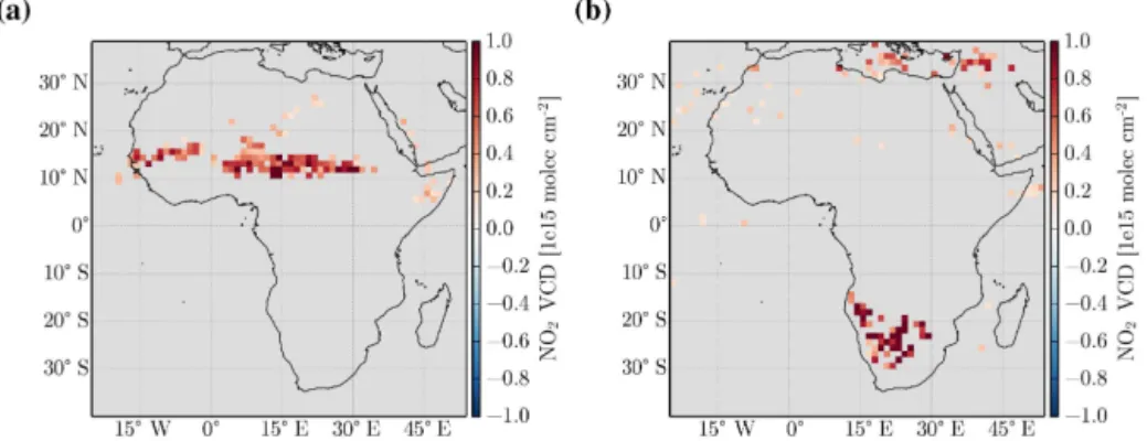
Figure 4. (a)Significant OMI NO2VCD enhancements (in 1×1015molec cm−2_{) on Day 0 compared to the background level for April–May–} June (2007–2010), which represents the start of the wet season after the dry period in the northern part of Africa. Extensive enhancements in NO2 over the narrow band of the Sahel can be seen.(b) The same for September–October–November (2007–2010), whereby strong enhancements are found in south-western Africa. This time period reflects the transition time between the dry and wet season in this region.

The most eminent features are the high enhancements of OMI NO2 column densities on Day 0 in the distinct band of the Sahel region around 15◦_{N. Single grid}

pix-els in this distinct band exceed absolute enhancements of 1×1015molec cm−2_{over background.}

Similar enhancements in the Sahel were also observed by Hudman et al. (2012). In the south-western part of Africa as well as over Australia spatially coherent enhancements are also present. Small-scale, local enhancements are found also, e.g. over India (also investigated by Ghude et al., 2010), re-gions nearby the Caspian Sea, the Middle East or China. An important finding is that there are no clustered reductions in NO2 VCDs on Day 0. Since we do not apply any land–sea mask, oceans serve as control regions for our algorithm: no significant differences in NO2 are found over the vast ma-jority of oceans area. However, over the Mediterranean sea and in proximity to coastal regions over oceans, small-scale enhancements in NO2VCDs are detectable, which might be related to advection.

The applied algorithm considers all data regardless of the season. Analysing the data based on different periods of the year reveals local enhancements in NO2VCDs in semi-arid areas matching dry-to-wet season transitions in these geo-graphic regions (Fig. 4). In April–May–June, Fig. 4a, the nar-row band of the Sahel again is characterized by a mean en-hancement of NO2of∼1×1015molec cm−2. This time

pe-riod corresponds to the start of the rainy season in the Sahel after a long dry spell of 3–4 months. In September–October– November, Fig. 4b, the strongest peaks in NO2 VCDs are observed in south-western Africa representing the start of the local wet season.

4.2 Detailed analyses over the Sahel region

The Sahel region represents a transition zone between the sa-vannah in the south and the Saharan desert in the north. It is characterized by a strong seasonality in rainfall governed by

the north–south movement of the inter-tropical convergence zone (ITCZ). The northward movement of the ITCZ starts in March and the northernmost position is reached, at 15◦_N,

in August. In the following four months the Sahel region receives about 90 % of its mean annual precipitation (Bell et al., 2000). The subsequent dry season begins in October and ends gradually with the start of the next wet season in April/May/June (AMJ period).

Previous studies (e.g. Jaeglé et al., 2004; Hudman et al., 2012) argue that in this distinct geographic band pulsed soil emissions of NOx, which can be detected from space, oc-cur at the beginning of the wet season in spring. Our findings support these previous studies and delineate this narrow band from 10 to 18◦_{N and from the west coast of Africa}

essen-tially spanning the whole width of the continent, as shown in Fig. 4a. The pronounced sNOxfeatures in the band of the Sahel during the AMJ period enable a more detailed investi-gation of pulsed soil emissions.

We restrict our detailed analysis to the central and eastern part of the Sahel region (0–30◦_{E, 12–18}◦_{N), similar to}

pre-vious studies (i.e. Jaeglé et al., 2004; Hudman et al., 2012). The western part of the Sahel shows a slightly weaker NO2 response to rain pulses, which might be related to different inter-annual variability patterns and seasonal cycles of pre-cipitation regimes (Lebel and Ali, 2009).

(10)

(a) 0 1 2 3 4 5 6 7 8

Precipitation [mm day

-1]

TMPA CMORPH PERSIANN

10 9 8 7 6 5 4 3 2 1 0 1 2 3 4 5 6 7 8 9 10 Days before and after first rain event 0.060 0.065 0.070 0.075 0.080 0.085 0.090 0.095 0.100 ESA v olumetric soil moisture [m m ] 3

-3 _{Soil moisture}

Soil moisture

(b) 0 1 2 3 4 5 6 7 8

-1]

10 9 8 7 6 5 4 3 2 1 0 1 2 3 4 5 6 7 8 9 10 Days before and after first rain event 0.60 0.65 0.70 0.75 0.80 0.85 H2

O VCD [1e23 molec cm

-2]

H

2

O VCD

GOME-2 H2O

(c) 0 1 2 3 4 5 6 7 8

-1]

10 9 8 7 6 5 4 3 2 1 0 1 2 3 4 5 6 7 8 9 10 Days before and after first rain event 38.0 38.5 39.0 39.5 40.0 40.5 Temperature [ C ]

Air temperature at 1000 hPa

Air temperature

(d)

10 9 8 7 6 5 4 3 2 1 0 1 2 3 4 5 6 7 8 9 10 Days before and after first rain event 6.5 7.0 7.5 8.0 8.5 9.0 9.5 10.0 10.5 11.0 Absolute humidity [g m ] -3

Humidity at 1000 hPa

Absolute humidity 12 14 16 18 20 22 24 R el at iv e h u m id it y [\ % ] Relative Humidity (e) 0 1 2 3 4 5 6 7 8

-1]

10 9 8 7 6 5 4 3 2 1 0 1 2 3 4 5 6 7 8 9 10 Days before and after first rain event 0.8 1.0 1.2 1.4 1.6 NO2

VCD [1e15 molec cm

-2]

NO

2

VCD

SCIAMACHY GOME-2 OMI (f) 0 1 2 3 4 5 6 7 8

-1]

10 9 8 7 6 5 4 3 2 1 0 1 2 3 4 5 6 7 8 9 10 Days before and after first rain event 3.5 4.0 4.5 5.0 5.5 6.0 6.5 7.0

HCHO VCD [1e15 molec cm

-2]

HCHO VCD

SCIAMACHY GOME-2 OMI

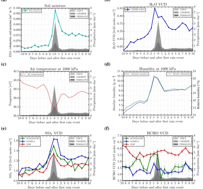
Figure 5.Temporal evolution of several quantities around the day with the first rain event for the Sahel region after at least 60 days of drought for April/May/June (2007–2010). Grey shaded areas represent precipitation estimates from TMPA, CMORPH and PERSIANN.(a)Blended ESA CCI soil moisture.(b)Water vapour total column densities from GOME-2.(c)Temperature at 1000 hPa from ECMWF Interim Analysis. (d)Relative and absolute humidity at 1000 hPa from ECMWF Interim Analysis.(e)NO₂VCDs from SCIAMACHY, GOME-2 and OMI with standard mean error (SME).(f)HCHO VCDs from SCIAMACHY, GOME-2 and OMI with SME.

missed or assessed differently by the individual data prod-ucts. Nevertheless, considering CMORPH or PERSIANN data as trigger leads to comparable responses in trace gases around the first day of rainfall (Appendix A).

The immediate wetting of the dry surface on Day 0 is cap-tured well by satellite observations of the volumetric soil moisture content as seen in Fig. 5a. After the initial wet-ting of the soil, the moisture content drops quickly during the following 3 days due to infiltration and evaporation. Sim-ilar behaviour is observed for total column densities of water vapour from GOME-2 in Fig. 5b. Water vapour content in the atmosphere gives insight into the ambient humidity and may indicate impending rain events, as humidity in the

(11)

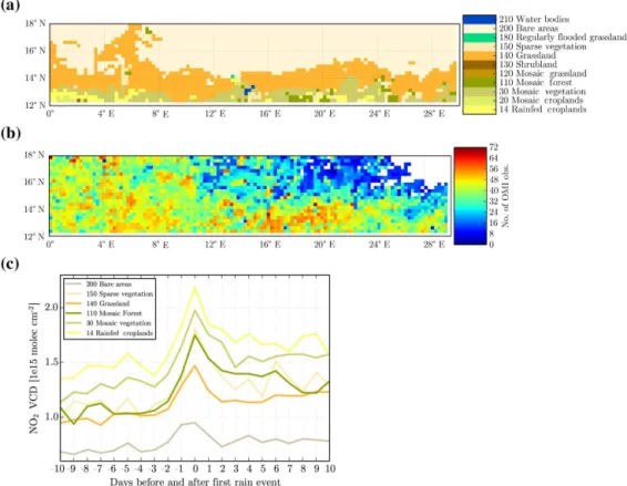
Figure 6. (a)ESA GLOBCOVER land cover classification for the Sahel downscaled to 0.25◦_×_0.25◦_{resolution with the corresponding}

(official) identification number, short name and colour information for each class.(b)Spatial location and number of OMI observations for the reference case analysis (AMJ, 2007–2010).(c)Rain-triggered NO2enhancements from OMI for the Sahel region separated by the dominant land cover types.

the mean (SME) value is indicated for each instrument and is generally smaller for OMI, which has the best statistics.

The average absolute enhancement in the Sahel for GOME-2 NO2 on Day 0 compared to the background lev-els is about 5×1014molec cm−2_{, whereas OMI and} SCIA-MACHY only observe an absolute enhancement of∼3 and 4×1014molec cm−2, respectively.

The different magnitudes of the enhancements cannot be solely explained by differences in overpass time or pixel size as GOME-2 and SCIAMACHY are similar in both aspects. Furthermore, higher emissions are expected in the afternoon, i.e. at OMI overpass time, when the temperature is higher. The corresponding SCDs, however, (see Fig. 9e) indicate that the differences seen in the NO2VCDs are mainly caused by differences in the AMF calculation for the three data prod-ucts.

Note that the enhancement is about 5×1014molec cm−2 on average, while it was shown in the previous section that for single 1.25◦

boxes the absolute enhancements can be as high as∼1×1015molec cm−2_{. Smaller grid pixels show} en-hancements of up to∼4×1015molec cm−2_{, and for single} events even larger enhancements are found.

Another striking feature, similar to the results for soil moisture, water vapour and precipitation, is the generally

higher NO2VCDs during the 10 days following the first rain-fall event compared to the background levels before Day 0. In Sect. 4.4 and 4.5, this important finding is studied more in detail by analyzing the NO2levels after Day 0 depending on wind conditions and the precipitation on Day+1 and beyond. As indicated in the introduction chapter, HCHO emissions from soils were found in several laboratory and field ex-periments (e.g. Veres et al., 2014). In Fig. 5f we also anal-ysed HCHO VCDs from OMI, SCIAMACHY and GOME-2 for potential pulsed emissions triggered by precipitation. The time series of HCHO for the three instruments, however, show no significant enhancement around the day of the first rain event. Possible reasons are the low signal-to-noise ratio for HCHO observations or very low emission rates.

4.3 Land cover analysis

(12)

300 m resolution to the 0.25◦_×_0.25◦ _{grid using a}

most-common-value method. The resulting land cover map is shown in Fig. 6a.

For different land cover types, both the NO2response on Day 0 and the background level of NO2vary systematically, see Fig. 6c. The observed NO2background VCDs per land cover type in the Sahel are mainly governed by biogenic emissions from soils and biomass burning. Anthropogenic activity and related emissions such as domestic fires or fertil-ized fields are at a very low level, and originate mostly from the southern, more populated part of the Sahel (Delon et al., 2010).

Systematic variations among the different land cover types are captured well: barren land, for example, shows the lowest levels of NO2compared to all other land cover types. Barren land relates to deserts with very low nitrogen input resulting in low sNOx, even after wetting. This land type is also associ-ated with fewer rainfall events, see Fig. 6b. Mosaic land cov-ers (a mixture between various vegetation types, grassland, cropland or forest), refer in this area to the loose term savan-nah delineating the transition zone between tropical forests and deserts. Savannahs can comprise various land cover sub-types and are characterized by distinct dry and wet periods with strong vegetation density and productivity during the wet season in summer. It is expected that savannah and cul-tivated land used for agriculture show strongest responses to initial rain events due to their higher potential for soil emis-sions. Figure 6c confirms these hypotheses: the largest NO2 enhancements are found for cropland and savannah; grass-land shows a significant, but smaller response; and the dri-est land cover type (bare area) shows only slightly enhanced NO2on Day 0.

4.4 Influence from other sources on the NO2signal

In this section, we investigate the effects of possible addi-tional sources of NOxsuch as fire or lightning and systematic errors in the satellite retrieval due to, e.g., changes in cloud fraction. To minimize the influence of these effects, our al-gorithm excludes measurements where lightning, fires or an effective cloud fraction>20% are detected.

4.4.1 Lightning NOx

Lightning is a natural source of NO2 in the upper tropo-sphere (e.g. Schumann and Huntrieser, 2007, and references therein). Since lightning typically occurs in high convective clouds that may correlate with the first rain event, our analy-sis is potentially affected.

Figure 7 depicts daily time series for NO2 VCDs, pre-cipitation and lightning counts averaged for the years 2007 to 2010. The seasonal evolution of the number of lightning strikes closely follows the precipitation patterns. Figure 7 also illustrates that lightning is not a governing source of NOxin the Sahel as no correlation between lightning strikes

0.25 0.75 1.25

NO

2

V

C

D Sahel

Ocean

50 100 150

Fire

1 3 5

Precip.

1 2 3 4 5 6 7 8 9 10 11 12 500

1500 2500

Lightning

Figure 7.Daily time series for the Sahel region (0–30◦_{W, 12–}

18◦_{N) averaged for the years 2007, 2008, 2009 and 2010. The}

first row of each panel shows mean NO₂ VCDs from OMI in molecules cm−2 _{(black) and a clean ocean reference (grey, 130–} 150◦_{W, 12–18}◦_{N). The second row shows the number of active}

fire counts in the Sahel from MODIS. The third row shows average precipitation from the TMPA/TRMM product in mm. The fourth row shows the number of lightning strikes detected by WWLLN.

and NO2VCDs can be found, although a direct proportion-ality would be expected. Precipitation also does not correlate well with the observed seasonal cycle in NO2. This is, how-ever, expected as microbial emissions of NOxfrom soils are not a linear function of soil moisture content or precipitation. Figure 8 shows results for the reference case, similar to Fig. 5, but with (solid lines) and without (dashed lines) light-ning screelight-ning; i.e. grid pixels coinciding with a lightlight-ning event are removed. Because of the low DE of the WWLLN in African regions (∼20 %) the lightning screening is also tested for central Australia (15–30◦

W, 2–10◦

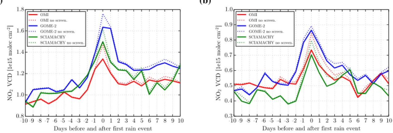
S) where the DE of the WWLLN is very high (80–90 %). Turning off the lightning screening leads to very similar results as for the reference case, but with a slightly stronger response in NO2VCDs on Day 0 for all three instruments. While this en-hancement might be partly caused by the additional NOx pro-duced by lightning, also a larger number of true precipitation-triggered events that lead to soil emissions may be included in this analysis. This is conceivable as clouds and thunder-storms accompanied by lightning strikes lead to the most heavy precipitation events. As the screening only causes mi-nor changes in peak NO2columns, lightning can be excluded as the main cause of the observed NO2enhancements.

4.4.2 Fire

The seasonal cycle in fire counts, depicted in Fig. 7, shows the highest activity in the Sahel in October and November for the years 2007 to 2010, while average NO2VCDs are the highest in summer.

(13)

(a)

10 9 8 7 6 5 4 3 2 1 0 1 2 3 4 5 6 7 8 9 10 Days before and after first rain event 0.8

1.0 1.2 1.4 1.6 1.8

NO2

VCD [1e15 molec cm

-2]

OMI OMI no screen. GOME-2 GOME-2 no screen. SCIAMACHY SCIAMACHY no screen.

(b)

10 9 8 7 6 5 4 3 2 1 0 1 2 3 4 5 6 7 8 9 10 Days before and after first rain event 0.3

0.4 0.5 0.6 0.7 0.8 0.9 1.0

NO2

VCD [1e15 molec cm

-2]

OMI OMI no screen. GOME-2 GOME-2 no screen. SCIAMACHY SCIAMACHY no screen.

Figure 8.Effect of lightning screening on the response of NO2VCDs around the first day of rainfall after a prolonged dry spell.(a)NO2 VCDs for the Sahel region from SCIAMACHY, GOME-2 and OMI without lightning screening (dashed lines) and with lightning screening (solid lines).(b)The corresponding results for central Australia (15–30◦_{W, 2–10}◦_S).

results in no change of the NO2signal (not shown). This is due to the fact that only very few fires occur in the wet sea-son, on average only in 0.002 % of all individual time series on Day 0 in the reference case, excluding fire as an important NO2source within our analysis.

4.4.3 Cloud effects

We have investigated possible cloud effects on our results by analyzing the temporal evolution of the mean cloud fractions (CF), NO2 VCDs and NO2 SCDs around the precipitation event. The latter was added as it provides the actual mea-sured signal without involving a tropospheric AMF, which is generally very sensitive to clouds.

Figure 9a depicts the mean effective CF for SCIA-MACHY, GOME-2 and OMI for the Sahel region. The dif-ferences of the absolute value of the CF are probably re-lated to the different cloud algorithms between GOME-2/SCIAMACHY (FRESCO+) and OMI (OMCLDO2). The

different temporal variation might also be partly related to the different overpass times and pixel sizes among the three satellite instruments. From these results we conclude that the observed NO2 peaks around Day 0 are not caused by cloud effects for the following reasons: first, for all sen-sors only small cloud fractions (<11 %) are found (for mea-surements with CF<0.2). Second, for SCIAMACHY and GOME-2 observations no systematic temporal variation of the CF is found. Third, the small but systematic enhance-ment of the CF around Day 0 found in the OMI observations would rather lead to a decrease (due to the shielding effect) of the NO2SCDs around Day 0 as soil emissions are expected to remain close to the surface. If only measurements with cloud fractions>20 % are considered, no spike is observed in the SCDs (Fig. 9f); GOME-2 and OMI even show a dip on Day 0, which is also seen in the respective VCDs (Fig. 9d). Interestingly, while there is a strong systematic enhancement of the FRESCO+ and OMCLDO2 cloud fractions, the NO2

SCDs show no peak around Day 0 for GOME-2 and OMI. This indicates that clouds effectively shield the pulsed soil emissions.

4.4.4 Influence of transport processes

Finally the possible influence of transport processes, which might be correlated with the occurrence of the first rain event, is investigated. As depicted in Fig. 10, a strong southerly wind is blowing at ground level (1000 hPa) the two days be-fore the first rain event and on Day 0 in the Sahel. In order to investigate whether polluted air from southern locations, es-pecially the tropics, is transported northward into the Sahel, we repeat the analysis for days governed by either northerly or southerly winds (Fig. 11). For the distinction between both directions we require that wind vectors from ECMWF at three different altitudes (600, 850 and 1000 hPa) point to the same direction in either case. The left panel in Fig. 11 de-picts results for northerly winds; the right panel for southerly winds. Although the background levels of NO2are reduced on days with northerly winds, enhancements in VCDs around the first day of rainfall remain apparent despite low statis-tics, especially for OMI and GOME-2 observations. For days with southerly winds the background is slightly higher and clear spikes for the OMI and GOME-2 observations can also be detected. Hence, these findings indicate that atmospheric transport has a systematic influence on the background NO2 levels (see also Sect. 4.5), but not substantially on the en-hancement around Day 0.

4.5 Latitudinal background correction and emissions after Day 0

(14)

Figure 9.Investigation of cloud effects on the retrieved NO₂SCDs and VCDs.(a)Mean cloud fraction of the three satellite instruments for the reference case (cloud fraction<20 %).(b) Mean cloud fraction of the three satellite instruments but considering only observa-tions with cloud fraction>20 %.(c)NO2VCDs for the reference case.(d) NO2 VCDs only considering observations with high cloud cover (cloud fraction>20 %).(e)NO2SCDs for the reference case.(f)NO2SCDs only considering observations with high cloud cover (cloud fraction>20 %).

by the precipitation-triggered sNOx pulsing event and, thus, can be used as reference to derive an absolute enhancement in NO2VCDs predominantly induced by pulsed soil emis-sions. However, it is shown in Figs. 5e and 9c, e that the NO2 VCDs after the pulsing event (Day+3 to Day+10) are con-sistently higher compared to the background before Day 0. This could be related to inflow of soil NOxfrom adjacent pix-els, which receive the first rain shortly after. However, initial tests showed that the number of such incidents is quite small (less than 5 %). For this reason, and because the effect is

(15)

10 9 8 7 6 5 4 3 2 1 0 1 2 3 4 5 6 7 8 9 10 Days before and after first rain event 1000

850 600

Pressure level [hpa]

u=1ms;v=0ms

Figure 10.Mean ECMWF wind vectors at three different pressure levels. At the surface, a strong south-westerly wind is blowing the 2 days before the first rain event in the Sahel region followed by northerly winds. At 600 hPa winds are constantly from the north-west.

This leads to four interesting questions. (i) Are the slightly enhanced NO2 VCDs after Day 0 related to the pulse on Day 0? (ii) In case the enhanced NO2VCDs after Day 0 are (partly) caused by other sources, what effect does a back-ground correction have on the retrieved absolute enhance-ments in NO2VCDs around Day 0? (iii) Is continuous pre-cipitation the cause for the enhancement after Day 0? (iv) In case the enhanced NO2VCDs after Day 0 are only related to the pulsed rain event, can we give quantitative estimates on these “continuous” soil emissions?

Figure 12a depicts the reference case analysis for the Sahel region with respect to 120 days around the first day of rain-fall after the drought period. The NO2 VCDs observed by the three satellite instruments show consistent patterns in the spike around Day 0 and still slightly enhanced NO2 VCDs 60 days after Day 0.

To investigate whether the increased NO2 VCDs after Day 0 are related to the pulsed rain on Day 0 or caused by a general change of the background NO2VCDs (e.g. related to a seasonal variation), we try to estimate the temporal evo-lution of the background (not affected by a pulsed rain event) in the following.

In a first attempt NO2VCDs are averaged over all grid pix-els located at the same latitude as the identified rain events as-suming latitudinal homogeneity in NO2background VCDs. This assumption is justified in the Sahel due to the latitudi-nal distribution of its land cover types governing NO2VCDs (the corresponding results are depicted in Fig. 12b). While compared to Fig. 12a, a much smoother temporal evolution is found (because more data are averaged), but apart from the much smaller spike on Day 0, very similar values can be seen in both panels. This confirms our assumption that the main part of the increase of the background value is not caused by the precipitation on Day 0. However, the spike in NO2VCDs around Day 0 is still evident because this averaging method

still considers the initial pixel with its adjacent neighbours, which are probably affected by either the overall precipita-tion pattern or spatial aliasing effects during the gridding of the NO2data products. Thus, in Fig. 12c a 10 pixel buffer is additionally applied to the algorithm. Screening out such pixels leads to a time series of NO2without the distinct spike around Day 0.

The time series of NO2VCDs retrieved using the two lati-tudinal averaging methods is denoted as the prevailing back-ground and is subsequently subtracted from the reference case analysis (Fig. 12). In the first case, without the appli-cation of an additional buffer (Fig. 12d), absolute enhance-ments of 0.43×1015molec cm−2 _{for GOME-2 and} SCIA-MACHY are found on Day 0. Also a steady increase in NO2 VCDs several days prior to Day 0 is observed. Although the pronounced spike in NO2 VCDs decreases rapidly in the days following Day 0, it lasts several weeks until the VCDs reach a minimum (but stays still slightly higher than on Day−60 to Day−20). A similar behaviour is observed for the case study with buffer screening (Fig. 12e). Here, ab-solute enhancements of 0.4×1015molec cm−2_{for OMI and} 0.62×1015molec cm−2_{for GOME-2 and SCIAMACHY are} found on Day 0.

(16)

(a) 0 1 2 3 4 5 6 7 8

-1] TMPA CMORPH PERSIANN

10 9 8 7 6 5 4 3 2 1 0 1 2 3 4 5 6 7 8 9 10 Days before and after first rain event 0.8 1.0 1.2 1.4 1.6 1.8 2.0 NO2

VCD [1e15 molec cm

-2] SCIAMACHY GOME-2 OMI (b) 0 1 2 3 4 5 6 7 8

-1] TMPA CMORPH PERSIANN

10 9 8 7 6 5 4 3 2 1 0 1 2 3 4 5 6 7 8 9 10 Days before and after first rain event 0.8 1.0 1.2 1.4 1.6 1.8 2.0 NO2

VCD [1e15 molec cm

-2]

Figure 11.Same as Fig. 5d, but filtered for(a)northerly and(b)southerly winds. The filter criterion is fulfilled, if the wind direction at 600, 850 and 1000 hPa is north or south, respectively.

same latitude. The changes on Fig. 13c are even smaller be-cause the pixels in proximity to the triggered rainy pixel are excluded from the averaging. Finally, Fig. 13d and e depict the differences between panel a and panels b and c, respec-tively. As expected, the enhancements in NO2VCDs around Day 0, are more pronounced for cases including a 10 pixel buffer during the background correction. Although the abso-lute enhancement on Day 0 is almost identical for the differ-ent cases, the time series still differ in the observed back-ground NO2 VCDs. These systematic differences, seen in Fig. 13d and e, hint at more complex variations in the back-ground, which are not entirely resolved by our correction. They could also be related to the fact that for the cases with longer dry periods after Day 0 the probability of precipita-tion in the vicinity of the considered locaprecipita-tion is lower. This implies, again, also differences in space and time of the ob-servations, which influences the observed NO2VCDs.

Generally, we find that the NO2VCDs stay enhanced af-ter Day 0 for a period of about 2 weeks, almost independent from the duration of the dry period after Day 0. This gives rise to the assumption that the enhanced emissions are mostly caused by the initial rain event on Day 0. Here, only results for OMI are presented because it has best statistics. Nev-ertheless, the analysis with data from the other instruments leads to the same conclusion.

4.6 Further study regions

As could be seen in the global analysis in Fig. 3, large-scale hot-spots in NO2VCD enhancements are not only detectable in the Sahel, but also in south-western Africa and in Aus-tralia. Subsequently, we present also the average NO2VCDs around the first day of rainfall for all three satellite instru-ments in these two regions.

Figure 14a depicts the results for south-western Africa (17–23◦_{E, 22–28}◦_{S) for a drought period}

(precipita-tion<2 mm) of at least 60 days in the months September– October–November 2007–2010 representing the transition

phase between the dry summer and following wet season. Compared to the Sahel reference case, the evolution of NO2 VCDs before and after the first day of rainfall increases and decreases more gradually without having a distinct spike on Day 0. This might be due to different environmental condi-tions such as soil type or lower statistics because of the much smaller spatial extent. It is, thus, more difficult to estimate the absolute enhancement compared to a defined background level. The difference between highest and lowest NO2VCDs in the full time series is∼0.5×1015molec cm−2_{for all three} instruments.

Figure 14b shows the analysis results for NO2 VCDs for the central part of Australia (120–145◦_{E, 22–31}◦_{S) for the}

time series from 2007 to 2010. Since the seasonality in rain-fall in this region is less pronounced, the full time series is considered in the analysis. The well pronounced spikes show an absolute enhancement of∼0.3×1015molec cm−2_{for the} three instruments, which is comparable to the findings from the Sahel and south-western Africa.

5 Discussion

5.1 Estimated nitrogen emission fluxes from the emission pulse

(17)

(a)

60 50 40 30 20 10 0 10 20 30 40 50 60 Days before and after first rain event 0.6

0.8 1.0 1.2 1.4 1.6

NO2

VCD [1e15 molec cm

-2] SCIAMACHYGOME-2 OMI

(b)

0.8 1.0 1.2 1.4 1.6

NO2

VCD [1e15 molec cm

(c)

0.8 1.0 1.2 1.4 1.6

NO2

VCD [1e15 molec cm

(d)

0.0 0.1 0.2 0.3 0.4 0.5 0.6 0.7

NO2

VCD [1e15 molec cm

-2] OMI_GOME-2

SCIAMACHY

(e)

0.00.1 0.2 0.3 0.4 0.5 0.6 0.7

NO2

VCD [1e15 molec cm

-2] OMI_GOME-2

SCIAMACHY

Figure 12.Analysis of NO2VCDs 60 days before and after the first day of rainfall in the April–May–June period for the Sahel region. (a)NO₂VCDs from OMI, GOME-2 and SCIAMACHY.(b)Latitudinal averaged NO₂VCDs corresponding to the reference (for details see text). (c)Latitudinal-averaged NO2VCDs corresponding to the reference considering an additional buffer of 10 pixels around the actual-triggered pixel to avoid influence of enhanced NO₂VCDs in the vicinity of the precipitation events.(d)Background corrected NO₂ VCDs:(a–b).(e)Background (with buffer) corrected NO2VCDs:(a–c).

pulsed soil emissions of NOxin the Sahel region and finds a comparable magnitude (49 % relative increase of OMI NO2 VCDs on Day 0) and length of the pulsing event (1–2 days) following the first rainfall. Here, we provide further evidence supporting that and other reported studies, i.e. the observed enhancements in NO2VCDs are consistent for multiple in-struments and are not introduced by retrieval errors or inter-fering sources.

For the Sahel region we find significant mean enhance-ments on the first day of rainfall in April–May–June averaged over four seasons (2007–2010) of ∼4×1014molec cm−2_, as observed by OMI, after the prolonged dry spell. How-ever, we see much stronger enhancements for single

pix-els on the original fine resolution grid (0.25◦_{) of up to} ∼4×1015molec cm−2_{. Considering these values as upper} and lower limits for the sNOx enhancement on Day 0, we can estimate emission fluxes. The top-down emission flux for NOx can be inferred from the NO2 VCD by mass bal-ance: E=NO2/τNO2 with NO2, being the tropospheric

NO2 VCD and τNO2 the lifetime. The lifetime for τNO2

(18)

(a)

0.8 1.0 1.2 1.4 1.6

NO2

[1e15 molec cm

-2]

0 days 3 days 5 days 10 days 20 days

(b)

0.8 1.0 1.2 1.4 1.6

NO2

[1e15 molec cm

-2]

0 days lat.avg. 3 days lat.avg. 5 days lat.avg. 10 days lat.avg. 20 Days lat.avg.

(c)

0.8 1.0 1.2 1.4 1.6

NO2

[1e15 molec cm

-2]

0 days lat.avg. 3 days lat.avg. 5 days lat.avg. 10 days lat.avg. 20 days lat.avg.

(d)

0.0 0.1 0.2 0.3 0.4 0.5 0.6

NO2

[1e15 molec cm

-2]

(e)

0.0 0.1 0.2 0.3 0.4 0.5 0.6

NO2

[1e15 molec cm

-2]

Figure 13.Investigation of the effect of different periods of dry days following Day 0.(a)Reference case analysis for OMI NO2VCDs filtered for time series experiencing 0, 3, 5, 10 and 20 days of drought after Day 0.(b)Background time series of NO₂VCDs without buffer screening as presented in Fig. 12b for the corresponding time series experiencing 0, 3, 5, 10 and 20 days of drought after Day 0.(c)The corresponding background time series of NO₂VCDs with buffer screening as presented in Fig. 12c.(d)Differences between panels(a, b). (e)Differences between panels(a, c).

65 ng N m−2_s−1_{on the upper limit on Day 0. This is in line} with findings from Jaeglé et al. (2004), who gave an estimate of 20 ng N m−2_s−1_{for rain-induced sNO}

x pulses in June in the Sahel. Furthermore, field studies suggest emission fluxes of nitrogen of about 2–60 ng N m−2_s−1_{(Johansson and} San-hueza, 1988; Davidson, 1992a; Levine et al., 1996; Scholes et al., 1997), which covers our estimated upper and lower limits. Previous studies also note the strong dependence of soil emissions on temperature. We conducted initial tests us-ing ECMWF soil temperature data (see Appendix F), but found no clear temperature dependence of sNOxemissions. This is probably due to the systematic relation between tem-perature and the seasonal cycle, which affects the

spatio-temporal selection of the data, e.g. in April more southern pixels are selected and in June more northern pixels. In con-sequence, we indicate the need for more detailed investiga-tion on how these pulsed emissions are affected by different soil temperatures.

(19)

(a) 0 1 2 3 4 5 6 7 8

-1]

10 9 8 7 6 5 4 3 2 1 0 1 2 3 4 5 6 7 8 9 10 Days before and after first rain event 0.81.0 1.2 1.4 1.6 1.8 2.0 2.2 2.4 NO2

[1e15 molec cm

-2] SCIAMACHY GOME-2 OMI (b) 0 1 2 3 4 5 6 7 8

-1]

10 9 8 7 6 5 4 3 2 1 0 1 2 3 4 5 6 7 8 9 10 Days before and after first rain event 0.3 0.4 0.5 0.6 0.7 0.8 0.9 1.0 NO2

[1e15 molec cm

-2]

Figure 14. (a)NO₂VCDs from SCIAMACHY, GOME-2 and OMI for south-western Africa in September–October–November around the first day of rainfall in this period. Precipitation is represented by the grey shaded areas.(b)Results for central Australia for the complete years 2007–2010.

potentially caused by the initial rain on Day 0 and not by sub-sequent precipitation the following days. Possible advection effects into or out of the considered pixels may thereby raise or lower the retrieved sNOx fluxes. The analysis based on different dry phases after Day 0 also changes the probability for first rain events in pixels in close proximity. As we do not find strong differences in the emissions for different dry phases after Day 0, we conclude that the inflow of NOxfrom adjacent pixels is not the dominant source for the enhance-ment after Day 0. In contrast, a systematic underestimation of the emissions is likely due to advection out of the central pixel. In sum, we estimate that the integrated emissions after Day 0 are potentially of the same order of magnitude as those from the first emission pulse on Day 0.

Peak emissions of sNOxpulses typically occur on the scale of 1–3 days (Kim et al., 2012) in accordance to our results for the Sahel, South Africa and Australia showing peak emis-sions shortly after the first re-wetting. Some studies, on the other hand, measure peak emissions several days after the first re-wetting of the soil, e.g. 7 days as observed in field by Oikawa et al. (2015). Our algorithm does not specifically distinguish between such cases by taking average time se-ries after the first precipitation event. Single pixels within the regions we investigated may exhibit peak emissions several days after the initial precipitation, which would, however, not be resolved by our analysis.

Our study focuses on the quantification of pulsed soil emissions and determines the NO2 enhancement on Day 0 and the following days with respect to a sophistically de-termined background. However, the seasonal pattern of the determined background, i.e. the NO2enhancement at the on-set of raining season (compare Jaeglé et al., 2004), clearly indicates that it is mainly driven by microbial emissions from soils as well: from pulsed emissions discarded by our strict selection criteria or continuous emissions dur-ing wet season. Note that the seasonal pattern of NO2 over the Sahel, as shown in Fig. 7, can neither be ex-plained by biomass burning nor lightning. Figure 13c of the

manuscript shows that the background NO2VCDs are about 0.9×1015molec cm−2_{. This is about 0}_.₁₇_×₁₀15_{molec cm}−2 higher than background in winter. Thus, in addition to the pulsed emissions quantified above, a mean background of 0.17×1015molec cm−2_{can be attributed to soil emissions as} well. These estimates are based on TMPA precipitation data. For other precipitation products (CMORPH or PERSIANN), results change only slightly (see Appendix E).

In summary, we discriminate between soil emissions within: (a) 1–3 days (initial peak), (b) 14 days and (c) sev-eral months (background during the wet season). The sepa-rate quantification of soil emissions belonging to these three categories might also be adopted in model parametrizations of soil emissions. However, further research needs to be con-ducted on how these emission categories vary for different regions worldwide.

5.2 Seasonal soil nitrogen emissions in the Sahel

In this section we quantify the total soil emissions, both due to pulsed emissions and background, for the Sahel region. For the pulsed emissions on Day 0 (category a) and the fol-lowing 2 weeks (b), the fluxes estimated above are multiplied by the area of the investigated region (0–30◦_{E, 12–18}◦_N).