Statistical Modeling of Manufacturing
Uncertainties for Microstrip Filters
Abraham E. Ortega P., Leonardo R.A.X. de Menezes and Humberto Abdalla Jr.
Dep. de Engenharia Elétrica, Faculdade de Tecnologia, Universidade de Brasília, Brasília-DF 70910-900 Brazil.
Abstract – This work presents a technique to characterize the errors that occur in the process of manufacturing into electromagnetic simulations of microwave devices. The procedure combines the unscented transform (UT) with simulations. The use of the UT allows efficient use of computational resources for the characterization of the random variables modeling the uncertainty. The technique was validated with the simulation, construction, and test of several sets of identical microstrip filters with very good results. Although the combination of UT and electromagnetic simulators was presented for microstrip filters, it can also be used for different types of microwave devices.
Index terms - Microstrip filters, Modeling, Monte Carlo methods,
Simulation software, Tolerance analysis.
I. INTRODUCTION
In the design and test of complex filters, electromagnetic simulation software is usually used for validation and accurate analysis. On the other hand, the manufacturing process introduces new sources of uncertainties into the assembled filter, which are difficult to model with the electromagnetic simulator. Thus, the result may present significant differences between measured and simulated responses, and this may reflect as increased cost in the final filter design.
Therefore, the accurate modeling of uncertainties in the manufacturing process has great potential to lead to better and shorter design cycles. The uncertainty is usually modeled using stochastic variables. In this representation, instead of a deterministic analysis of filter, it is better to perform a statistical study of the problem. The results are typically the expected value, the standard deviation and the confidence intervals of the response.
alternative technique is the Unscented Transform (UT), which can reduce the simulation problem substantially. The essential idea is based on the approximation of a continuous probability distribution by discrete one. Since the distribution is discrete, only a finite number of simulations will be necessary to get the statistics of the problem. Obviously, the goal is to use the discrete distribution with as few points as possible with the highest accuracy possible. Thus, the UT approach allows efficient use of electromagnetic simulation in the characterization of mapped random variables. In this paper, the UT technique was used to characterize the effects of error tolerance on the response of the assembled microstrip filter. This quantifies the effect of uncertainty in the assembled device still into the simulation stage.
The objective of this work is to show how to include the uncertainty of the manufacturing process into the electromagnetic simulation. The inclusion of these effects allows the estimation of which fabrication tolerances are critical, and the effects of several sources of uncertainty.
This work is organized as follows: Section II presents a brief review of the modeling of errors by continuous and discrete distributions. The major part of this section presents a general UT theory. The section finishes with its application in cases where the error is modeled by an uniform distribution. Section III presents the accuracy analysis of different electromagnetic simulators used to characterize a band pass, and band reject another. The cutoff frequency and bandwidth of these filters were the relevant parameters analyzed. Also in this section the simulators are ranked according to an assessment of the responses of the different filters. Section III closes with the presentation of the application of the Unscented Transform (UT) for the error modeling of the two filters. This analysis is done considering the major sources of uncertainty and comparing the statistics of the measured and simulated responses for each type of filter. Section IV draws the conclusions, and the last section suggests proposals for future work.
II. THEORY A – Modeling Error
As more variables are also subjected to the previously mentioned kind of error, then more random variables with suitable distributions are required. The addition of more variables raises the problem of interdependence between them. In this work, the variables were considered independent as a basic simplification. The characterization of the correlation between them is beyond the scope of this work. The introduction of new variables also causes some troubles with the uncertainty representation. The greater the number of variables, the greater the number of simulations required. In most cases this requirement grows exponentially [3].
The solution to this type of problem is to reduce the number of variables. This is done by identifying which are the most significant ones. The test requires different simulations for each of the variables independently. Once the main sources of uncertainty causing the major effects are identified, then only those variables will be used in the final simulation. In this work, this number was limited to two variables for each filter. Naturally, this is a necessary and common simplification.
In addition to the manufacturing error, there is also the numerical error. However, this error is either very difficult to quantify or geometry dependent. Although it seems amendable to treat this sort of uncertainty with random variables, the modeling of the distribution and representation of the error of such cases is still unclear. Therefore, in this work the effect of the numerical error was considered negligible when compared to other sources of error. Such assumption was enforced by an appropriate choice of the simulator. The procedure is detailed in section comparison between simulators.
B – Modeling a Continuous Distribution by a Discrete One
The effect of a variable x in a known process can be represented by a function G(x). This is exact provided that certain mathematical requirements such as smoothness and continuity are satisfied. However if ones wants to characterize the effect of the uncertainty of x in G(x), the problem is equivalent to the calculation of the statistical moments of the mapping G(û) when û is a random variable. If the function G(x) can be represented by its Taylor expansion [3], then a truncated polynomial representation can be written by:
∑
= = + + + + = n n n nx a x a x a x a a x G 0 3 3 2 2 1 1 0 ) ( ⋯ (1)Since the polynomial is truncated, that implies that the expected value of the mapping is:
{
}
∫
∑
∑
{ }
= = = = = k m m m k m mmu a Eu
a E du u p u G û G E 0 0 ) ( ) ( )
( (2)
{
}
∑
∫
=
= a u p u du û
G
E m
k
m
m ( )
) (
0 (3)
If the distribution is discrete, the expected value will be:
{
}
∑
∑
=
=
n m n n k
m
m p u
a û
G E
0
) (
(4) Where pn are the weights (probabilities) of the discrete distribution, and un are the sigma points
(discrete points of the distribution). The result of mapping will be equal provided that:
∫
=∑
n n m n m
p u du u p
u ( )
(5) Since the mapping has the same results for the discrete and continuous representation of û:
∫
∑
G u p = G u p u du nn
n) ( ) ( )
( (6)
The equation (6) shows that the moments to the mapped variable can be calculated either using a continuous or discrete distribution; the result will be the same provided that the moments of the two distributions are equal.
Since the discrete distribution only needs calculation at a finite number of points, this means that the moments of the mapped variable will be calculated in a simpler form if a discrete distribution is used.
C – The theory of UT
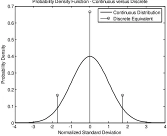
The UT was developed in 1997 by Julier and Uhlman [4] and is used in various areas of electrical engineering [5], [6]. One possible interpretation for the UT is of a discrete approximation of a continuous probability density function.
Since the discrete probability density function has only a few points then the number of simulations required is minimal. As highlighted in the previous section, an important requirement is that the discrete and continuous distributions [7] have the same moments.
-4 -3 -2 -1 0 1 2 3 4 0 0.1 0.2 0.3 0.4 0.5 0.6 0.7
Normalized Standard Deviation
P ro b a b il it y D e n s it y
Probability Density Function - Continuous versus Discrete
Continuous Distribution Discrete Equivalent
Fig. 1. Representation of the continuous normal distribution and discrete approximation.
The weights pn and un sigma points are fully available once the necessary moments are calculated.
Since (5) has to hold for all moments, the calculation of the weights and sigma points is the solution of a system:
{ }
{ }
∫
∑
∫
∑
= = = = = = du u p u û E p u du u up û E p u k k i n i k i i n i i ) ( ) ( 1 1 ⋮ (7)This system has to be truncated at some point. A satisfactory compromise is limiting the system up to the fourth moment. The main reason is that most tables usually present up to the kurtosis of the distribution.
Another useful simplification is to consider that distribution has zero mean and unitary variance. In this case this system of equations becomes:
1 3 1 0 1 2 1 4 1 1 3 1 2 1 = + = = = =
∑
∑
∑
∑
∑
= = = = = n i i n i i i n i i i n i i i n i i i p p u p u p u p uγ
γ
(8)Where γ1 is the skew of the continuous distribution and γ2 is the excess kurtosis. The discrete points
[
]
[
2]
1 2 1 3 2 2 1 2 1 1 3 ) 3 ( 4 2 1 0 3 ) 3 ( 4 2 1
γ
γ
γ
γ
γ
γ
− + + = = − + − = u u u (9)It remains only to find the weights:
[
][
2]
1 2 2 1 2 1 1 3 ) 3 ( 4 3 ) 3 ( 4 2
γ
γ
γ
γ
γ
− + − + −− =
p (10)
3
2
2 2 1 2 2 1 2−
−
−
−
−
=
γ
γ
γ
γ
p
(11)[
][
2]
1 2 2 1 2 1 3 3 ) 3 ( 4 3 ) 3 ( 4 2
γ
γ
γ
γ
γ
+ + − + −− =
p (12)
Although the calculations were performed for zero mean, unit variance distributions, the generalization for other cases is simple. If u is a random variable with mean U and standard deviation
σ, the sigma points are:
[
]
[
γ γ γ]
σσ γ γ γ 2 1 2 1 3 2 2 1 2 1 1 ) ( 3 ) 3 ( 4 2 1 ) ( 3 ) 3 ( 4 2 1 − + + + = = − + − + = U S U S U S (13)
D – Applying the UT to the Uniform Distribution
Once the probability distribution is determined, the sigma points and weights are easily calculated. The sigma points and weights for the case of the uniform distribution in the interval [-1, 1] are presented in Tables I and II [8].
TABLE I. SIGMA POINTS FOR THE NORMALIZED UNIFORM DISTRIBUTION
n(order) Zeros (Normalized Sigma Points)
0 0
1 -0.577, 0.577
2 -0.77459, 0, 0.77459
3 -0.86114, -0.33998, 0.33998, 0.86114
TABLE II. WEIGHTS FOR THE NORMALIZED UNIFORM DISTRIBUTION
n(order) Weights
0 1
2 0.278, 0.444, 0.278
3 0.1740, 0.326, 0, 0.326, 0.1740
The combination of the UT with an electromagnetic simulator is exemplified as follows: a particular device has a single transmission line with an average width of 2.25mm with and an error of 0.1mm (uniform distribution). Using the second order UT, three simulations will be necessary [9] as shown in Table III.
TABLE III. POINTS OF SIGMA APPROACH TO ONE VARIABLE
Number of simulations Width of gap (mm)
1 2.25
2 2.25– 0.775*0.05 = 2.21125
3 2.25+ 0.775*0.05 = 2.28875
So far, only single variable distributions were considered. What about multivariable ones? The way to solve this problem depends if the distribution are independent or not. If all the variables are independent, then the problem is solved in the same manner of the continuous case. Several sources of uncertainty will require several random variables.
As a first example one can consider a problem with two independent random variables, both with zero mean and a uniform distribution. If we use the UT of first order then the set of sigma points in this case is: (-0.577, -0.577), (-0.577, 0.577), (0.577, -0.577) e (0.577, 0.577) and each has a weight of 0.25 (the product of 0.5 to 0.5). This results in 4 simulations.
Naturally as one seeks greater accuracy, it becomes necessary to use higher orders, which require more simulations (for instance, a second order requires nine simulations). If instead of a single line, as in the case described in Table III, the problem has now two lines modeled as independent variables (both with zero mean and uniform distribution) the result is a combination of 3 by 3 sigma points (2nd order - total of 9). The results are presented in Table IV.
TABLE IV. POINTS OF SIGMA APPROACH TO TWO VARIABLES
Number of simulations Width of Gap 1 (mm) Width of Gap 2 (mm)
1 2.25– 0.775*0.05 = 2.21125 2.25– 0.775*0.05 = 2.21125
2 2.25– 0.775*0.05 = 2.21125 2.25
3 2.25– 0.775*0.05 = 2.21125 2.25+ 0.775*0.05 = 2.28875
4 2.25 2.25– 0.775*0.05 = 2.21125
5 2.25 2.25
6 2.25 2.25+ 0.775*0.05 = 2.28875
7 2.25+ 0.775*0.05 = 2.28875 2.25– 0.775*0.05 = 2.21125
8 2.25+ 0.775*0.05 = 2.28875 2.25
9 2.25+ 0. 0.775*0.05 = 2.28875 2.25+ 0.775*0.05 = 2.28875
loss, bandwidth, center frequency, and so on. The UT allows the calculation of a number of statistical parameters, but in this work the main ones are expected value, standard deviation and cumulative distribution function (which allows to characterize the confidence interval) of the device subject to uncertainty.
Since there are a very large number of variables that may be sources of uncertainty, it is important to define what the most important ones are. The UT also provides magnitude information on which variables are responsible for random variations in the response, and how many random variables are needed for the model. This is possible using the statistical correlation and marginal statistical properties of multiple random variables [9].
One simple form to determine the most relevant variables is to determine the proportion of variation. If x and y are two variables, one may use the proportion:
} { } {
} { }
{ } {
} {
y Var x Var
y Var or
y Var x Var
x Var
+
+ (14)
This equation provides an approximate relationship between the significance of the variables.
Once the solutions to the set of sigma points are calculated, the results can be combined according to weighted average calculation described in the UT theory to provide a good estimate of the moments of the mapped distribution.
Naturally, the performance of uncertainty modeling using the UT is as good as the simulation tool itself. For this reason the next section begins with a comparison of results from different electromagnetic software packages.
III. RESULTS
1- COMPARISON BETWEEN DIFFERENT SIMULATORS
As discussed in section I, the UT was used to model manufacturing errors at the simulator stage instead of at the prototype stage. The main assumption is that the simulator response is a very good approximation of the one of the ideal device (without assembly errors). Naturally, that is not always true.
Therefore it is necessary to check the magnitude of the numerical errors involved in each problem. Unfortunately the value of the numerical uncertainty may be somewhat dependent on the problem. In this work two different types of microstrip filters were assembled (one band pass and one band stop). The band pass filter was designed with a center frequency of 1.8 GHz and 150 MHz bandwidth. The band stop one were designed with a center frequency of 1.8 GHz and a 1 GHz bandwidth. Both type of filters were designed for microstrip technology with a substrate of relative permittivity εr = 10 and
thickness h = 1.57mm.
standard FDTD simulator (free in the Internet). One of numerical techniques of CST (FITD) is similar to FDTD, but the CST has other numerical techniques implemented on it.
These reference simulations were then compared to the average result of measurements of the prototypes. The purpose of the comparison was to determine which simulator had the best response in comparison to the measurements. Naturally, all programs had their strong and weak points, so a score was devised to rank the response of each simulator. The simulations were compared to the average result of the measurements for each type of filter.
The goal of making this comparison is to choose a simulator that effectively covers most of the parameters to be simulated. It is also an objective to demonstrate that all simulators have an intrinsic error in the simulation, which can modify slightly the output response.
In fact, two additional filters based on different topologies were built. The choice of the simulation tool was based on the overall response of the four different filters. The filters that are presented in this work were chosen for its implementation and simplicity in the manufacturing process (one based on gap coupling, and the other on stub resonance).
A – Dual-mode ring gap resonator band pass filter
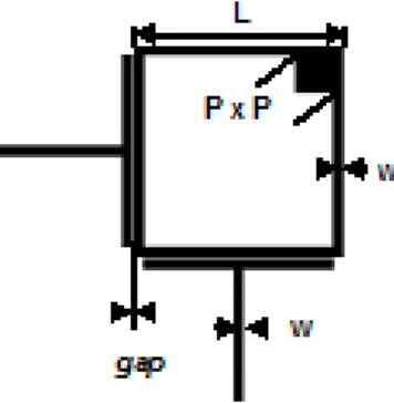
The first test was the simulation of dual-mode ring gap resonator with a disturbance, as shown in Fig. 2. The introduction of disturbance allows that two modes are present within a single resonator.
Stronger coupling, ie, smaller gap, resulted in a narrowing of the bandwidth, and increased disturbance (p value) resulted in an increase in the bandwidth [10].
All six filters have the same characteristics; each filter should be equal to the other with the same process of assembly. The construction method is described in [13]
This filter was designed for 1.8 GHz of center frequency and a bandwidth of 150 MHz. The width w of the lines in the resonator ring is 1 mm and width of the coupling gaps is 0.2 mm. The disturbance p is 2.5 mm, the size of L is 17.6 mm.
Fig. 2. Layout of the filter pass-band dual-mode in ring fed by the gaps.
0 0.5 1 1.5 2 2.5 3 -70
-60 -50 -40 -30 -20 -10 0
Frequency (GHz)
In
s
e
rt
io
n
l
o
s
s
(
d
B
)
Comparison between Average, FDTD, SONNET and CST.
Average Simulation FDTD Simulation SONNET Simulation CST
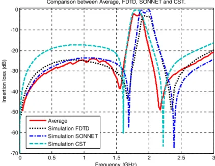
Fig. 3. Comparison between Average, FDTD, SONNET and CST.
A.1 - Center Frequency
Fig.3 shows that there are differences of the center frequency between the measured (average) and simulated curves. Nevertheless, the CST simulation curve approximates the measurement curve better. This is also presented in Table V.
TABLE V. CENTRAL FREQUENCY –FILTER 1
C. Frequency (GHz) Lag(GHz)
Average 1.82 0.00
FDTD 1.97 0.15
SONNET 1.94 0.12
CST 1.81 0.01
This indicates that the center frequency was better calculated by the CST simulator, and the other simulators are a bit off, because they follow the same trend of the average.
A.2 – Bandwidth
The bandwidth is better represented in Table VI.
TABLE VI. BANDWIDTH –FILTER 1
Bandwidth (GHz) Difference (GHz)
Average 0.174 0.00
FDTD 0.199 0.025
SONNET 0.185 0.011
CST 0.156 0.018
In order to have an overall impression of the performance of each simulator, a scoring scheme was devised: the best result would be ranked 3 and the worst result 1. After the score was calculated for each parameter, an overall mean was determined.
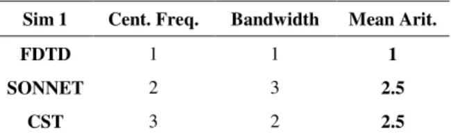
An analysis was also performed to determine the overall score of this filter. The results are summarized in Table VII. The conclusion is that the CST and SONNET had equal scores.
TABLE VII. SCORE BEHAVIOR OF THE SIMULATORS
Sim 1 Cent. Freq. Bandwidth Mean Arit.
FDTD 1 1 1
SONNET 2 3 2.5
CST 3 2 2.5
Given the different results found in the review of this filter, when comparing the simulated curves of the three simulators, and the average, one can reaches the conclusion that CST and SONNET had a better score than the FDTD simulators.
B – Stub-Loaded Filter
The second example used filter with a geometry consisting of a wide central stub and lateral thin stubs [11] as shown the Fig. 4.
Fig. 4. Layout of the Filter band stop.
0 0.5 1 1.5 2 2.5 3 -60
-50 -40 -30 -20 -10 0
Frequency (GHz)
R
e
tu
rn
L
o
s
s
(
d
B
)
Comparison between Average, FDTD, SONNET and CST
Average
Simulation FDTD Simulation SONNET Simulation CST
Fig. 5. Results for the return loss of the band stop filter
Fig 5 emphasizes the rejection band because this band provides more information and better clarity regarding the simulation results.
There are some differences between the curves, but the main shape of the curve remains the same for measurement and simulations.
B.1 - Central Frequency
The filter was designed for a center frequency of 1.8 GHz. By observing Fig. 5, it is clear that this value is practically the same in all curves. Nevertheless there is a small difference between them, which can be seen in Table VIII.
TABLE VIII. CENTRAL FREQUENCY –FILTER 2
C. Frequency (GHz) Lag(GHz)
Average 1.78 0.00
FDTD 1.69 0.09
SONNET 1.773 0.007
CST 1.76 0.02
Table VIII shows the results of three simulators and are very close to the average center frequency. However the SONNET e CST simulators results closer to measurements when compared to FDTD
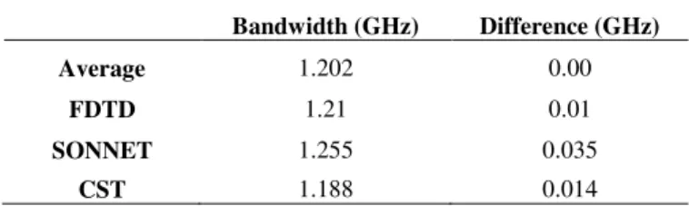
When looking at Fig. 5 one can see that the bandwidths are of similar size with respect to the average, nevertheless there is little difference between them as can be seen in Table IX.
TABLE IX. BANDWIDTH –FILTER 2
Bandwidth (GHz) Difference (GHz)
Average 1.202 0.00
FDTD 1.21 0.01
SONNET 1.255 0.035
CST 1.188 0.014
Table IX shows that the FDTD simulator presented the best bandwidth results. The next best result was from the CST program. The score is presented in Table X. As it may be seen, the CST simulator displayed better performance in this case.
TABLE X. SCORE BEHAVIORAL OF THE SIMULATOR
Sim 2 Cent. Freq. Band Arit Mean.
FDTD 1 3 2
SONNET 3 1 2
CST 2 2 2
An important lesson is that the accuracy of the simulator was very dependent on the size of the filter. This dependency had a tendency to decrease as simulation parameters were refined.
C – Which simulator presented better fidelity?
Table XI summarized the scores of the simulators for all filters. Although, no simulator package proved to be a complete solution, the CST package displayed better overall results in comparison to the other packages. It should be noted, that if commercial full versions of the programs were used, maybe the differences would not be so clear.
TABLE XI. FINAL RESULTS OF SIMULATOR COMPARISON
Final Score Sim. 1 Sim. 2 Arit. Mean
FDTD 1 2 1,5
SONNET 2.5 2 2.25
CST 2.5 2 2,25
The second important point is that even though the UT approach coupled with electromagnetic simulation assumes that the major source of error is the manufacturing, this is certainly not always the case. The simulation process has an intrinsic error that might be larger than the other sources of error. However all electromagnetic simulators have intrinsic errors due to the type of numerical method that uses, but these errors in most of times are negligible.
The same geometry of the filter was analyzed by each simulator; however the convergence of each one was different. In this particular subject, the simulator CST presented better convergence.
Therefore, the CST program did show certain advantages in comparison to others because its results, its simulation speed, and its flexibility in the variation of parameters.
The topology of these filters was carefully chosen because of the different filtering principles. In the first filter, the gap coupling is instrumental for the filter response. In the second filter, the stub resonance is the main mechanism. These two filters summarize the basic ideas used in simple parameters (gap width and stub length/position).
2.-. RESULTS OF THE UTAPPLICATION
As mentioned before, the main of objective of this work is the statistical characterization of device behavior at the simulation stage. The statistical characterization consisted in obtaining the expected value, standard deviation and cumulative probability function (CDF). The calculation of the CDF used the techniques developed in [12]. The manufacturing technique is a thermal transfer system described in detail in [13].
1- Analysis of the gap ring resonator band pass filter
A - Sources of uncertainty.
Fig. 6. Band Pass ring-fed dual-mode constructed filter.
B - Measurements and Simulations.
Figure 7 shows the six prototypes measurement curves, and it also shows the nine simulated curves (because of the nine required sigma-points for second order accuracy).
0 0.5 1 1.5 2 2.5 3
-70 -60 -50 -40 -30 -20 -10 0
Frequency (GHz)
In
s
e
rt
io
n
L
o
s
s
(
d
B
)
Comparison between Measurement and Simulations
Meas. 1 Meas. 2 Meas. 3 Meas. 4 Meas. 5 Meas. 6 Simu. 1 Simu. 2 Simu. 3 Simu. 4 Simu. 5 Simu. 6 Simu. 7 Simu. 8 Simu. 9
Fig. 7. Comparison between measurement and simulation of a ring fed dual mode filter.
0 0.5 1 1.5 2 2.5 3 0
1 2 3 4 5 6 7 8 9 10
Frequency (GHz)
In
s
e
rt
io
n
L
o
s
s
(
d
B
)
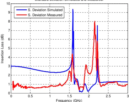
Standard Deviation Simulated and Measured.
S. Deviation Simulated S. Deviation Measured
Fig. 8. Comparison between measured and simulated magnitude standard deviation of ring fed dual mode filter
Figure 8 indicates that there is high sensitivity on the magnitude near cutoff frequencies (both in simulation and measurement). The analysis allows one to conclude that the measurements and the behavior of UT are in good agreement; however one can make a deeper analysis using the CDF for several parameters that will be shown below.
C - Analysis of Results
C.1 - Center Frequency
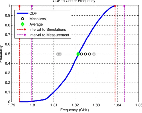
1.790 1.8 1.81 1.82 1.83 1.84 1.85 0.1
0.2 0.3 0.4 0.5 0.6 0.7 0.8 0.9 1
CDF to Center Frequency.
Frequency (GHz)
P
ro
b
a
b
ili
ty
CDF Measures Average
Interval to Simulations Interval to Measurement
Fig. 9. CDF to Center Frequency.
Figure 9 shows that the oscillation is well distributed with respect to the expected value (corresponding to the point of 50% probability); therefore the modeling of errors is satisfactory. Although the measurements are not evenly distributed, all are within the confidence interval.
The confidence interval is estimated at 95% between 1.806 and 1.837 GHz.
C.3 – Bandwidth
The CDF of the bandwidth is presented in Fig. 10.
0.110 0.12 0.13 0.14 0.15 0.16 0.17 0.18 0.19 0.2 0.21
0.1 0.2 0.3 0.4 0.5 0.6 0.7 0.8 0.9 1
CDF to Bandwidth
Frequency (GHz)
P
ro
b
a
b
ili
ty
CDF Measures Average
Interval to Simulations Interval to Measurement
Figure 10 shows that most of the measured points are within the 95% confidence interval. However, the two points outside this interval suggests that either the simulator response has some intrinsic errors, or that there are additional sources of error that were not modeled.
The confidence interval is estimated at 95% and that between 0.1467 and 0.1711 GHz.
2 - Analysis with the stub-loaded band stop filter.
A - Sources of Uncertainty.
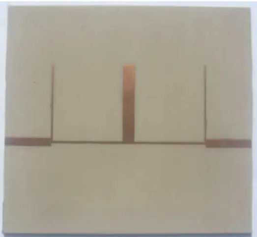
This filter had a simple geometry, so the sources of uncertainty are likely to be either the width or position of stubs, Fig. 11. After a series of tests it was found that changing the distance between stubs caused significant change to the results.
Fig. 11. Band Stop Filter Constructed.
B - Measurements and Simulations.
0 0.5 1 1.5 2 2.5 3 -70
-60 -50 -40 -30 -20 -10 0
Frequency (GHz)
R
e
tu
rn
L
o
s
s
(
d
B
)
Comparison between Measurement and Simulation
Meas. 1 Meas. 2 Meas. 3 Meas. 4 Meas. 5 Meas. 6 Simu. 1 Simu. 2 Simu. 3 Simu. 4 Simu. 5 Simu. 6 Simu. 7 Simu. 8 Simu. 8
Fig. 12. Comparison between Measurement and Simulation.
The results show that the simulated central frequency and bandwidth are very close to the measurements.
0 0.5 1 1.5 2 2.5 3
0 2 4 6 8 10 12
Frequency (GHz)
R
e
tu
rn
L
o
s
s
(
d
B
)
Standard Deviation Simutated and Measured
S. Deviation Simulated S. Deviation Measured
Fig. 13. Standard Deviation Simulated and Measured.
C - Analysis of Results
C.1 - Center Frequency
It is readily seen in from Fig. 14, that all the measurements are contained in the 95% confidence interval defined by the CDF.
1.75 1.76 1.77 1.78 1.79 1.8 1.81
0 0.1 0.2 0.3 0.4 0.5 0.6 0.7 0.8 0.9 1
CDF to Center Frequency
Frequency (GHz)
P
ro
b
a
b
ili
ty
CDF Measures Average
Interval to Simulations Interval to Measurement
Fig. 14. CDF to Central Frequency.
The confidence interval is estimated at 95% and that between 1.758 and 1.796 GHz.
C.3 – Bandwidth
1.18 1.185 1.19 1.195 1.2 1.205 1.21 1.215 1.22 0
0.1 0.2 0.3 0.4 0.5 0.6 0.7 0.8 0.9 1
CDF to Bandwidth
Frequency (GHz)
P
ro
b
a
b
ili
ty
CDF Measures Average
Interval to Simulations Interval to Measurement
Fig. 15. CDF to Bandwidth.
The confidence interval is estimated at 95% and the frequency ranges between 1.18 and 1.208 MHz. The numerical and measured results for the two filters are presented in Table XII.
TABLE XII. SUMMARY OF ALL SIMULATIONS AND MEASUREMENTS
First Filter Second Filter
C. Freq. Band C. Freq. Band
Measured 1 1.953 0.127 1.792 1.195
Measured 2 1.935 0.152 1.785 1.198
Measured 3 1.968 0.134 1.775 1.199
Measured 4 1.939 0.146 1.777 1.191
Measured 5 1.959 0.159 1.766 1.200
Measured 6 1.943 0.141 1.769 1.189
Average 1.949 0,143 1.777 1.195
Deviation 0.013 0.012 0.009 0.005
Simulation 1 1.955 0.132 1.797 1.187 Simulation 2 1.919 0.142 1.785 1.188 Simulation 3 1.941 0.156 1.775 1.197 Simulation 4 1.903 0.148 1.756 1.179 Simulation 5 1.919 0.162 1.776 1.184 Simulation 6 1.933 0.144 1.783 1.189 Simulation 7 1.954 0.162 1.762 1.199 Simulation 8 1.948 0.152 1.793 1.194 Simulation 9 1.957 0.152 1.772 1.208
Average 1.932 0.151 1.777 1.189
The data show that the measured and simulated responses are statistically consistent regarding the average result and the standard deviation. This is a clear indication that the CST program coupled with the UT approach successfully modeled the effect of manufacturing uncertainties in this case.
IV. CONCLUSIONS
Through this work presented a new simple and accurate technique for characterization of uncertainties by UT coupled with electromagnetic simulators. This approach presents the UT as a statistical consistent form to include the uncertainties produced in the manufacturing process in the electromagnetic simulation.
The validation of this method was performed including the effects of uncertainty in the simulation and comparing the effects with real measurements of the filters. The results indicate that the combination of UT and EM simulator can characterize accurately the effects of uncertainty.
The curves of the results provide suitable validation of the technique. The approach can be used to improve the design models, shorten production cycles and add external effects (such as corrosion or aging) for the electromagnetic simulation.
Because the technique is based on precise characterization of the sources of uncertainty, a study of various simulators was implemented. The objective was to determine the simulation package with the most appropriate response for a particular type of filter. After several tests, the software package CST was chosen because of the fidelity of the response in the cases studied, compared with the measurements. This package was then used to model the effect of uncertainties.
As there are different simulators, using different numerical methods, there is some degree of variation in output response. This means that even simulated filter can produce different answers, depending on the simulator used.
An important conclusion is that all simulators introduce some kind of intrinsic error that may, under certain circumstances, emerge as a dominant mechanism in the final uncertainty. This means that even if the other sources of uncertainty are adequately modeled, it may happen that the simulator error ends up masking the final results when compared with measurements. Unfortunately, although this error might still be adequately modeled using the UT, the procedure to do so is not clear at this time. The results of the expected central frequency and bandwidth show that the UT can adequately model these parameters. This information is better represented by the CDF curve of the different filters. By observing the curves of the CDF, one can notice that the points representing the measurements are within the confidence interval and very close to the simulated expected value.
great accuracy. This can prevent the construction of several prototypes and possibly accelerate the final design to market.
V. FUTURE WORKS
As suggestions of future work, there are several studies that can be performed: the probability distribution function of the source of uncertainty has to be adequately characterized (this means building test structures to determine de cdf), other microstrip structures should also be analyzed by the UT, the UT could also be used to characterize active devices, and the concept of uncertainty modeling suggests that the use of a optimization process could lead to more robust designs.
ACKNOWLEDGEMENT
This work was supported by the Brazilian Research Agency (CNPq).
VI. REFERENCES
[1] Papoulis, Probability, Random Variables, and Stochastic Processes,. 3rd ed. New York: McGraw-Hill, 1991.
[2] Abraham E. Ortega P. Leonardo R.A.X. de Menezes “Äplicação da Transformada da Incereteza (UT) para Projetos de
Filtros de Microondas” University, Brazil, Feb. 2010.
[3] Leonardo R.A.X. de Menezes, Ajibola Ajayi, Chistos Chistopoulos, Fillip Sewell and Geovany A. Borges, “ Efficient Computation of Stochastic Electromagnetic Problems Using Unscented Transforms” Subbimeted to IEEE Trans. Of
Antennas and Propagation on May 4, 2007.
[4] 2S. J. Julier and J. K. Uhlmann, A general method for approximating nonlinear transformations of probability distributions Oxford, U.K.: Eng. Dept., Univ. Oxford, Tech. Rep.
[5] 3J.L. Crassidis and F. L. Markley, “Unscented filtering for spacecraft attitude estimation,” J. Guid. Control Dyn., vol.
26, pp. 536-542, 2003.
[6] 4L. Sige, Z. Xiaoxin, F. Mingtian, and Z. Zhuping, "Probabilistic Power Flow Calculation Using Sigma-Point Transform Algorithm," in the Proc. PowerCon 2006. Oct. 2006 Page(s):1-5
[7] Leonardo R.A.X. de Menezes, Ajibola Ajayi, Christos Christopoulos, Fillip Sewell and Geovany A. Borges, “Efficient
Extraction of Statistical Moments in Electromagnetic Problems Solve with of Method of Moments” Dep. De Engenharía Elétrica, Faculdade de Tecnologia, Universidade de Brasília, Brasília – DF 70910-900 BRAZIL, George Green Institute for Electromagnetic Research, Univ.of Nottingham, Nottingham NG7 2RD, U.K. May 2007.
[8] Leonardo R.A.X. de Menezes, Ajibola Ajayi, Chistos Chistopoulos, Fillip Sewell and Geovany A. Borges, “ Recent Advances in the Combination of the Unscented Transform (UT) with the Transmission Line Modeling Method (TLM)” Dep. De Engenharía Elétrica, Faculdade de Tecnologia, Universidade de Brasília, Brasília – DF 70910-900 BRAZIL,
George Green Institute for Electromagnetic Research, Univ.of Nottingham, Nottingham NG7 2RD, U.K. May 2007. [9] Leonardo R.A.X. De Menezes. Abraham Ortega Paredes. Humberto Abdalla Junior and Geovany A. Borges “Modeling
Device Manufacturing Uncertainty in Electromagnetic Simulations,” Dep. De Engenharía Elétrica, Faculdade de Tecnologia, Universidade de Brasília, Brasília – DF 70910-900 BRAZIL. June. 2008.
[11]Hong, J. S. and Lancaster, M. J., Microstrip Filters for RF/Microwave Applications. New York: Wiley, 2001.
[12]Edson A. da Costa Jr., Leonardo R. A. X. De Menezes, “Propagação de incertezas em eletromagnetismo” PhD Theses
in Electrical Engineering. Brasília University., Brazil, May2009.