www.atmos-chem-phys.net/11/6167/2011/ doi:10.5194/acp-11-6167-2011
© Author(s) 2011. CC Attribution 3.0 License.
Chemistry
and Physics
A new method to detect long term trends of methane (CH
4
) and
nitrous oxide (N
2
O) total columns measured within the NDACC
ground-based high resolution solar FTIR network
J. Angelbratt1, J. Mellqvist1, T. Blumenstock5, T. Borsdorff4, S. Brohede1, P. Duchatelet2, F. Forster4, F. Hase5,
E. Mahieu2, D. Murtagh1, A. K. Petersen3,*, M. Schneider5, R. Sussmann4, and J. Urban1
1Chalmers University of Technology, G¨oteborg, Sweden
2Institute of Astrophysics and Geophysics, University of Li`ege, Li`ege, Belgium 3Institute of Environmental Physics, University of Bremen, Bremen, Germany
4Karlsruhe Institute of Technology (KIT), Institute for Meteorology and Climate Research (IMK-ASF), Garmisch-Partenkirchen, Germany
5Karlsruhe Institute of Technology (KIT), Institute for Meteorology and Climate Research (IMK-ASF), Karlsruhe, Germany *present address: Max-Planck-Institute for Meteorology, Hamburg, Germany
Received: 21 December 2010 – Published in Atmos. Chem. Phys. Discuss.: 10 March 2011 Revised: 14 June 2011 – Accepted: 20 June 2011 – Published: 1 July 2011
Abstract. Total columns measured with the ground-based
solar FTIR technique are highly variable in time due to at-mospheric chemistry and dynamics in the atmosphere above the measurement station. In this paper, a multiple regres-sion model with anomalies of air pressure, total columns of hydrogen fluoride (HF) and carbon monoxide (CO) and tropopause height are used to reduce the variability in the methane (CH4) and nitrous oxide (N2O) total columns to estimate reliable linear trends with as small uncertainties as possible. The method is developed at the Harestua sta-tion (60◦N, 11◦E, 600 m a.s.l.) and used on three other European FTIR stations, i.e. Jungfraujoch (47◦N, 8◦E, 3600 m a.s.l.), Zugspitze (47◦N, 11◦E, 3000 m a.s.l.), and Kiruna (68◦N, 20◦E, 400 m a.s.l.). Linear CH4 trends be-tween 0.13±0.01-0.25±0.02 % yr−1were estimated for all stations in the 1996-2009 period. A piecewise model with three separate linear trends, connected at change points, was used to estimate the short term fluctuations in the CH4 to-tal columns. This model shows a growth in 1996–1999 followed by a period of steady state until 2007. From 2007 until 2009 the atmospheric CH4amount increases be-tween 0.57±0.22–1.15±0.17 % yr−1. Linear N2O trends between 0.19±0.01–0.40±0.02 % yr−1were estimated for all stations in the 1996-2007 period, here with the strongest trend at Harestua and Kiruna and the lowest at the Alp
Correspondence to:J. Mellqvist ([email protected])
stations. From the N2O total columns crude tropospheric and stratospheric partial columns were derived, indicating that the observed difference in the N2O trends between the FTIR sites is of stratospheric origin. This agrees well with the N2O measurements by the SMR instrument onboard the Odin satellite showing the highest trends at Harestua, 0.98±0.28 % yr−1, and considerably smaller trends at lower latitudes, 0.27±0.25 % yr−1. The multiple regression model was compared with two other trend methods, the ordinary linear regression and a Bootstrap algorithm. The multiple regression model estimated CH4 and N2O trends that dif-fered up to 31 % compared to the other two methods and had uncertainties that were up to 300 % lower. Since the multi-ple regression method were carefully validated this stresses the importance to account for variability in the total columns when estimating trend from solar FTIR data.
1 Introduction
Methane (CH4) and nitrous oxide (N2O) are among the largest contributors to the greenhouse effect (IPCC, 2007).
important CH4emission sources are ruminants, natural gas leakage and fossil fuel and biomass burning. The amount of CH4 in the atmosphere has increased during the later part of the twentieth century. Between 1978–1987 in situ measurements has shown that the growth rate was impor-tant, (i.e. 1.1 % yr−1), but during the late 1980 the growth rate was slowing down to 0.3–0.6 % yr−1 and even lower growth rates were reported during the 1990s (Simpson et al., 2006). In the early 2000s the CH4 growth rate was nearly zero. During 2007 and 2008 however, CH4 was on the rise again and global growth rates of 0.47±0.04 % yr−1 and 0.25±0.04 % yr−1 were reported each respective year (Dlugokencky et al., 2009).
In contrast to CH4, the dominant N2O source, both nat-ural and anthropogenic, is microbial activity in soils. The source is strongly linked with the use of synthetic nitro-gen fertilizers, which have increased during the later part of the twentieth century (Davidson, 2009). Other important N2O sources include: biomass burning, sewers, livestock and emission from transport and industries. The main sink for N2O is photodissociation in the stratosphere by ultravio-let light and reaction with excited oxygen atoms (Bates and Hays, 1967). Compared to the CH4trend, the N2O accumu-lation in the atmosphere has been continuous. During the last three decades, the atmospheric N2O burden has shown an al-most (constant) linear increase with a reported annual change of 0.26 % yr−1(IPCC, 2007).
This paper was carried out within the EU project HYMN (Hydrogen, Methane and Nitrous Oxide, http://www. knmi.nl/samenw/hymn/) and one of the goals was to im-prove and homogenize the CH4 and N2O retrievals from high-resolution solar FTIR (Fourier Transform Infra Red) measurements and to obtain, for both gases, total columns and vertical profiles as accurately as possible. Many of the participating ground-based FTIR stations have time se-ries that cover 15 years of data or more and it is therefore possible and interesting to study long term trends. Trends from greenhouse gases from FTIR measurements have ear-lier also been performed within the EU project UFTIR (http: //www.nilu.no/uftir/) (Vigouroux et al., 2008).
One advantage when using FTIR total columns for the es-timation of long term trends is their insensitivity to local vari-ations of the atmosphere. In addition, since the global circu-lation is zonal in the free troposphere and stratosphere, the air stays at approximately the same latitude and the measure-ment station will therefore represent the atmosphere at that latitude. Hence, only a few stations at different latitudes are needed to represent the whole atmosphere. One disadvantage with FTIR is the fact that the time series often are unevenly sampled since the solar absorption infrared measurements re-quire clear sky conditions. Furthermore there are, for some stations, periods of missing data due to instrument failure and for the most northern stations because of the polar winter.
One of the common methods for estimating trends of at-mospheric parameters is to use monthly average values (see
for example Jones et al., 2009). The use of this method re-duces the variability in the time series and removes the even-tual periods of missing data. For an evenly sampled time se-ries it is also possible to take the autocorrelation (also called serial correlation) into account (Tiao et al., 1990; Weath-erhead et al., 1998). The FTIR data are autocorrelated on different timescales e.g., caused by meteorological patterns, seasonal cycles and other kinds of long-term variability. This correlation can best be described as a memory in the time series where a value at a certain time contains information of earlier values. Since our present FTIR time series in-clude both unevenly sampling and in some instance signif-icant gaps it is difficult to create representative monthly av-erages. It is for some stations even impossible without in-terpolation. We use instead a multiple regression model, including a linear trend, a seasonal component and anoma-lies from various atmospheric parameters to account for the time series variability and autocorrelation to estimate reliable trends. The method also gives a possibility to quantify the atmospheric parameters that affect the measured time series through their contributions to the fitted regression model.
2 FTIR measurements and data retrieval
In this paper we use total column time series of CH4, N2O, carbon monoxide (CO), hydrogen fluoride (HF) and ethane (C2H6)measured with FTIR spectrometers at four European stations, i.e. Jungfraujoch, Zugspitze, Harestua and Kiruna, within the NDACC network (Network for the Detection of Atmospheric Composition Change, http://www. ndsc.ncep.noaa.gov/). FTIR measurements have been per-formed since the mid 1990s, both in the Northern and South-ern hemispheres. Information about the stations, instrumen-tations and retrievals are presented in Table 1. The CH4 and N2O trend analysis cover the 1996–2009 and 1996–2007 time periods, for respectively species.
All the FTIR spectrometers involved in this study oper-ate in the mid infrared spectral region from 700 cm−1 to 5000 cm−1(2 to 14 µm) and measure the molecular absorp-tion of solar light in the atmosphere for a wide range of species. Derived atmospheric abundance is expressed in terms of total column, defined as the sum of molecules from the top of the atmosphere down to the measurement station, per unit area (often expressed as molecules per square cen-timetre). To be able to spectrally resolve the atmospheric absorption lines for a given species, high resolution spec-trometers are needed. For the stations in this paper a typical spectral resolution of 0.0035–0.005 cm−1is used.
Table 1.FTIR stations included in the trend study.
Jungfraujoch Zugspitze Harestua Kiruna
Latitude (◦N) 47 47 60 68
Longitude (◦E) 8 11 11 20
Altitude (m a.s.l) 3600 3000 600 400 Instrument type Bruker 120HR Bruker 125HRa Bruker 125Mb Bruker 125HRc Retrieval code SFIT2 SFIT2 SFIT2 PROFFIT No. of measurement days, CH4 1135 818 599 642 No. of measurement days, N2O 1160 739 592 765
abefore 2006 Zugspitze operated a Bruker 120HR,bbefore 2008 Harestua operated a Bruker 120M andcbefore 2007 Kiruna operated a Bruker 120HR.
by varying the mixing ratio profile of the target species to-gether with interfering species such as H2O and CO2. In this manner vertical profile of the target species can be obtained. These are generally calculated into total columns using the available pressure and temperature information but for some species the data can also be divided into partial columns for instance dividing the total column into a tropospheric and stratospheric part. The height information available from the spectra is usually defined as the degrees of freedom (DOFs) which is obtained from averaging kernel calculations accord-ing the principles described by Rodgers (2000).
The retrievals in this paper are performed by the two algo-rithms SFIT2 (Rinsland et al., 1998) and PROFFIT (Hase et al., 2004). The two codes have been shown to be in excel-lent agreement with a deviation of only 1 % or less (Hase et al., 2004). To quantify the instrument performance regarding line broadening and phase shift gas-cell measurements are done regularly on all instruments. These measurements are evaluated with the LINEFIT program (Hase et al., 1999).
The CH4 and N2O retrievals are done with a common strategy developed within the EU project HYMN, where the micro-windows, spectroscopic line lists, retrieval parame-ters, sources of ancillary data like pressure-temperature pro-files, and water vapour data for deriving dry air columns are identical for all involved stations and used to minimize the biases between the stations.
In an earlier FTIR trend study by Gardiner et al. (2008), the retrievals were carried out by the optimal estimation al-gorithm (Rodgers, 2000). In this retrieval alal-gorithm a cost function is minimized which corresponds to a weighted com-bination of a multiple least square solution and the a priori information. In the case of CH4 and N2O severe oscilla-tions in the profiles are obtained and therefore instead a re-trieval algorithm based on Tikhonov regularization (Twomey, 1996) has been applied to minimize this problem. In the lat-ter retrieval algorithm, a cost function is minimized which corresponds to a weighted combination of a multiple least square solution and a cost term that corresponds to the first derivative of the vertical profile. The latter term min-imises oscillations of the retrieved profile versus height but
Table 2.Microwindows with interfering species used to retrieve the CH4and N2O total columns.
Species Microwindows (cm−1) Interfering species CH4 2613.70–2615.40 HDO, CO2
2650.60–2651.30 HDO, CO2 2835.50–2835.80
2903.60–2904.03 NO2
2921.00–2921.60 H2O, HDO, NO2
N2O 2481.28–2482.62 CO2, CH4
2526.40–2528.20 CO2, CH4, HDO
2537.84–2538.82 CH4
2540.00–2540.75 CH4
reduces the profile information to 2–3 independent partial columns (DOFs). For more information regarding FTIR re-trieval with Tikhonov see Sussmann and Borsdorf (2007) and Sussmann et al. (2005).
In Table 2 information regarding the HYMN micro win-dows and interfering species are presented. For both CH4 and N2O Hitran 2004 linelist parameters are used.
The CO, C2H6and HF total columns, used as atmospheric parameters in the multiple regression model, are retrieved with standard procedures that have earlier been developed within the NDACC community (Mellqvist et al., 2002) (De-Mazi`ere et al., 2005). The retrieval procedure varies slightly from site to site but uses consistent micro window regions for CO (2057–2159 cm−1), C2H6 (2976–2977 cm−1) and HF (4038–4039 cm−1).
3 The Odin satellite
and were performed time-shared with other operation modes on every third day until April 2007 and on every second day since then, providing a quasi-continuous N2O data set from 2001 to 2010. N2O in the stratosphere is retrieved between roughly 12–14 km and 60 km with a vertical resolution of about 1.5 km and a single-scan precision of 10–15 % (below 30 km). For the here relevant level-2 data version 2.1 See e.g. Murtagh et al. (2002); Urban et al. (2005b,a); Urban (2006); and Strong et al. (2008) for a description of the Odin mis-sion and information of the N2O measurements, error analy-sis and validation studies.
4 Trend method
4.1 Linear regression
Regression analysis is a technique to study the connection between a dependent variable and one or several independent variables. In this paper we mean the dependency between the independent variable, time, and the dependent variable, the measured total column time series. The simplest way to de-tect a trend is by fitting a straight line with the least squares method to the data, the slope of the line then represents the trend. The estimated trend itself is of limited use without an estimate of its error which could be represented with a confidence interval. When calculating a trend and its con-fidence interval three assumptions are usually made: (1) the residuals (measured-model) are assumed to be free from au-tocorrelation, (2) the distribution of the residuals is assumed to be approximately normally distributed and (3) the resid-uals are assumed to have equal variance. Large deviations from these assumptions will result in errors in the estimated trends and its confidence intervals (Weatherhead et al., 1998; Tiao et al., 1990). Methods have been developed to account for autocorrelation when estimating trends but they all need data which have equidistant time steps between the measure-ments. However, due to local weather conditions and avail-able sunlight hour’s time series derived from FTIR observa-tions are not sampled evenly and typically contain gaps. It is hence not possible to make representative weekly or monthly averages and thereby get time series with constant time spac-ing. To reduce the time series variability and estimate reliable trends a multiple regression model is used in this paper.
4.2 Atmospheric parameters
Several atmospheric parameters that are assumed to affect the measured total column of CH4and N2O are discussed in this section. Data from the Harestua station have been used to test the effect of various atmospheric parameters on the mea-sured total columns of CH4and N2O. The parameters that have shown to have a significant effect on the measured total columns of CH4and N2O at the Harestua station have then been applied to the FTIR data from the other participating stations.
Changes in theair pressuredue to meteorological fluctu-ations will change the amount of molecules above the mea-surement station. A high pressure is expected to result in a high total column and vice versa. CH4 and N2O have their highest partial columns close to ground level, where they are intensively produced, and are therefore expected to be very sensitive to fluctuations in the air pressure. Thetropopause heightis expected to affect the stratospheric column of CH4 and N2O but also to stretch and compress the tropospheric column. A low tropopause height is thought to make the tropospheric contribution to the total column smaller and a high larger. The tropopause height data used here are from the ECMWF (European Centre for Medium Range Weather Forecasts, http://www.ecmwf.int/) model that de-fines the tropopause altitude as the lowest level where the lapse rate is 2◦C km−1or less and no height within 2 km above this point exceeds this value. To account for the pres-ence of the polar vortex a range ofPV (polar vorticity) val-ues, at different altitudes (10–25 km), is obtained from the ECMWF model. A high PV value is expected to correspond to the presence of vortex air above the measurements site and hence a low stratospheric column of CH4and N2O.
The total column of the stratospheric species HF has been used in several other studies, among them Toon et al. (1997) and Mellqvist et al. (2002), as a proxy for stratospheric transport. This transport involves the downward motion of airmasses when the station is inside the polar vortex, the changes in tropopause height and the vertical and horizontal motion of air masses in the stratosphere. Hence, a largetotal column of HF is expected to result in a large stratospheric and a small tropospheric column of CH4and N2O.
CH4, N2O, CO and C2H6 are all produced in fossil fuel and biomass burning. Thetotal columns of CO and C2H6 are therefore used as a proxy for large scale biomass burn-ing events as the ones present in Canada and Russia durburn-ing the summers of 1998, 1999, 2002 and 2003 (Yurganov et al., 2004,2005). Thetotal columns of C2H6will in addition be used as a proxy for natural gas leakage. This has, as to our knowledge, not been tested on CH4and N2O FTIR total columns before.
Other physical parameters that have been investigated are: the number of sunspots, the North Atlantic Oscilla-tions (NAO) and the Quasi Biennial OscillaOscilla-tions (QBO).
4.3 Trend model
of 12 months. The 12 month seasonal cycle is strongest at the high altitude stations due to the well mixed air i.e. the low influence of local sources. A more advanced represen-tation of the seasonal cycle, a third order Fourier series, has also been tested in the model but did not improve the model compared to the basic one. To explain the time series vari-ability, i.e. short term deviations from the background trend and seasonal fluctuations, anomalies derived from some of the atmospheric parameters described in Sect. 4.2 are used. These anomalies correspond to the detrended and deseason-alized time series of the atmospheric parameters.
To find the anomalies that affect the CH4 and N2O total columns all derived anomalies are inserted into the multiple regression model, presented in Eq. (1), and tested with the stepwise regression method. This means that the combina-tion of anomalies that gives the best adjustedR2 value and are statistically significant are used in the final trend model and all the others being excluded. We define statistically sig-nificant as a parameter for which the confidence interval ex-cludes zero on a 2-σlevel.
To estimate trends the anomalies found with the stepwise approach, the background trend and the seasonal component are inserted in the model in Eq. (1) and solved with the least squares method.
y=β0+β1sin(2π t )+β2cos(2π t )+ I
X
i=3
βia(t )i−2
+βI+1t+βI+2(t−cp1)A+βI+3(t−cp2)B+ε
where
t >cp1,A=1
t≤cp1,A=0
t >cp2,B=1
t≤cp2,B=0
(1)
Wheretis the time in fraction of years and cp1 and cp2 are change points when the trend is expected to change direc-tion or magnitude. For CH4, possible change points in 1999 and 2007 have been reported by Dlugokencky et al. (2003, 2009) who have made global in situ measurements. In a first trend estimation no change points will be used for CH4and N2O while in a second estimation the change points of Dlu-gokencky et al. (2003, 2009) will be used for CH4. When no change points are used only the first trend term in Eq. (1) will be present in the model. In Eq. (1)y is the dependent variable (CH4or N2O) andβ corresponds to the regression coefficients. Thea(t )i terms represent the anomalies from the atmospheric parameters (i to I) andεis the residual or un-explained part of the model. The term is assumed to be nor-mal distributed with a constant variance around zero and free from auto correlation. In the regression model the anomalies,
a(t )i,tandymust all be of the same length. This means that for a certain day in the CH4or N2O time series there must exist corresponding data for all of the calculated anomalies.
1996 1998 2000 2002 2004 2006 2008 2010
1.4 1.6 1.8 2 2.2 2.4 2.6 2.8
x 1018
C
O
t
o
ta
l
co
lu
m
n
(
m
o
le
cu
le
s
cm
-2)
Year
Measured Fitted model
1996 1998 2000 2002 2004 2006 2008 2010
-4 -2 0 2 4 6
x 1017
C
O
t
o
ta
l
co
lu
m
n
(
m
o
le
cu
le
s
cm
-2)
Year
Anomalies
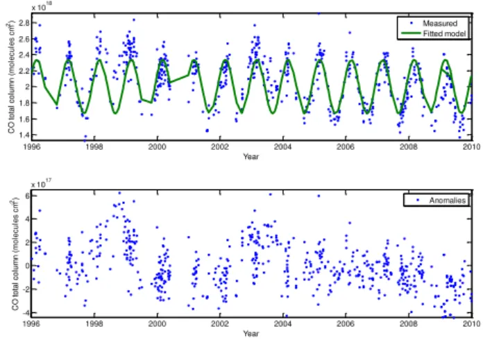
Fig. 1. Measured total column of CO at Harestua with fitted model (upper panel) and calculated anomalies (lower panel). To ob-tain the anomalies the fitted model is subtracted from the measured time series.
To estimate confidence intervals for the trends a method for hypothesis testing described by Montgomery et al. (2008) is used.
4.4 Deriving anomalies
To obtain anomalies from the atmospheric parameters pre-sented in Sect. 4.2, a model consisting of a seasonal func-tion and a polynomial with varying order is fitted to each of the atmospheric parameters, Eq. (2). The fitted model is then subtracted from the original atmospheric time series. To find the optimal polynomial fit for each atmospheric parame-ter the adjustedR2value is used (Montgomery et al., 2008). The value reflects the correlation between the model and the measurements and adjusts this correlation to the number of terms used in the regression model. If no adjustment is used the correlation always increase when increasing the number of terms in the regression model, this favours over fitting. An adjustedR2value close to one indicates a small residual and a good model fit while zero indicates the opposite.
y=β0+β1sin(2π t )+β2cos(2π t )+β3t+β4t2+β5t3 (2) In Eq. (2)yis the dependent variable i.e. the atmospheric pa-rameters (air pressure, tropopause height and so on) andβ
5 Results
5.1 Anomalies in the final regression model
The anomalies shown to affect the measured total columns of CH4 are: the air pressure, the total column of CO and HF and the anomalies that affect the N2O total columns are: the air pressure the total column of HF and the tropopause height. The air pressure, CO and tropopause height anoma-lies are derived using Eq. (2) along with a linear trend. For HF a second order polynomial is used in Eq. (2) for Harestua, Jungfraujoch and Zugspitze while a linear trend is used for the fit of the Kiruna dataset.
The stepwise regression model that was applied on the Harestua data showed a final model where C2H6where in-cluded instead of CO, this due to a slightly higher adjusted
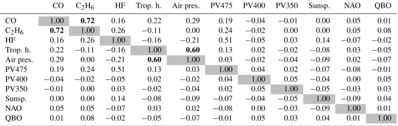
R2value. At the time of performing the stepwise test not all stations were retrieving C2H6. Instead CO has to be used in the final model. Since C2H6and CO shows a strong correla-tion this practical simplificacorrela-tion was assumed to work prop-erly. The linear correlations between all the tested anomalies are presented in Table 3. Except the CO-C2H6correlation a slightly weaker correlation can be seen for the air pressure and the tropopause height. The other anomalies have much weaker or no linear correlations.
The final regression coefficients of the stepwise regression model for Harestua are presented in Table 4. In the table it can be seen that the air pressure and the total column of HF and CO is significant for both CH4and N2O. PV375 is also significant for CH4and the tropopause height is significant for N2O. Although their significance not all parameters are included in the final model due to the fact that the adjusted
R2value not is improved.
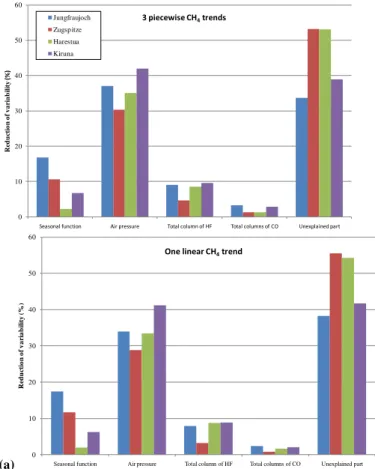
The reduction of the variability in the CH4and N2O time series due to the addition of anomalies are presented in Fig. 2a and b, respectively. The reduction is calculated by comparing the standard deviation of the residuals when only offset and linear trend/trends is fitted to the data with the stan-dard deviations derived when each of the anomalies and the seasonal function is added to the trend model. The seasonal function accounts for a few to roughly 18 % of the variabil-ity of the two CH4 cases. The value is slightly higher for N2O which show up to 22 %. For both species the seasonal function has the greatest impact at Jungfraujoch and smallest at Harestua. In the two CH4cases the air pressure anomaly accounts for 30–40 % of the variability. The corresponding value for N2O is roughly 30 %. The HF anomaly reduces the variability more for N2O,∼11–18 %, than for CH4,∼2– 10 %. The anomalies from CO and tropopause height corre-sponds both to a variability reduction of a couple of percent each. There is still place for improvements in the trend model since 30–55 % of the variability is unexplained, depending on station and species. This has partly to do with the mea-surement noise from the instrument but most likely also with atmospheric processes not captured in this paper.
0 10 20 30 40 50 60
Seasonal function Air pressure Total column of HF Total columns of CO Unexplained part
R
ed
u
ct
io
n
o
f
v
a
ri
a
b
il
it
y
(%
)
3 piecewise CH4trends
Jungfraujoch
Zugspitze
Harestua
Kiruna
t
(a)
0 10 20 30 40 50 60
Seasonal function Air pressure Total column of HF Total columns of CO Unexplained part
R
ed
u
ct
io
n
o
f
v
a
ri
a
b
il
it
y
(
%)
One linear CH4trend
Fig. 2a.Reduction of the variability in the CH4time series from the
anomalies and seasonal function in the regression model, presented as percent of total variability. The upper panel is when three piece-wise trends are used and the lower is when a single linear trend is used.
(b)
0 10 20 30 40 50 60
Seasonal function Air pressure Tropopause height Total column of HF Unexplained part
R
ed
u
ct
io
n
o
f
v
a
ri
a
b
il
it
y
(
%)
One linear N2O trend
Jungfraujoch
Zugspitze
Harestua
Kiruna
Fig. 2b.Reduction of the variability in the N2O time series from the anomalies and seasonal function in the regression model, presented as percent of total variability.
Table 3.Linear correlation calculated from the anomalies at the Harestua site. Correlations stronger or equal to 0.60 is marked in bold.
CO C2H6 HF Trop. h. Air pres. PV475 PV400 PV350 Sunsp. NAO QBO CO 1.00 0.72 0.16 0.22 0.29 0.19 −0.04 −0.01 0.00 0.05 0.01 C2H6 0.72 1.00 0.26 −0.11 0.00 0.24 −0.02 0.00 0.00 0.05 0.08 HF 0.16 0.26 1.00 −0.16 −0.21 0.51 −0.05 0.03 0.14 −0.07 −0.02 Trop. h. 0.22 −0.11 −0.16 1.00 0.60 0.13 0.02 −0.02 −0.08 0.03 −0.05 Air pres. 0.29 0.00 −0.21 0.60 1.00 0.03 −0.02 −0.04 −0.09 0.02 −0.07 PV475 0.19 0.24 0.51 0.13 0.03 1.00 0.04 0.02 −0.07 −0.08 −0.01 PV400 −0.04 −0.02 −0.05 0.02 −0.02 0.04 1.00 0.05 −0.04 0.00 0.05 PV350 −0.01 0.00 0.03 −0.02 −0.04 0.02 0.05 1.00 −0.05 −0.03 0.03 Sunsp. 0.00 0.00 0.14 −0.08 −0.09 −0.07 −0.04 −0.05 1.00 −0.09 0.04 NAO 0.05 0.05 −0.07 0.03 0.02 −0.08 0.00 −0.03 −0.09 1.00 0.01 QBO 0.01 0.08 −0.02 −0.05 −0.07 −0.01 0.05 0.03 0.04 0.01 1.00
(a)
1996 1998 2000 2002 2004 2006 2008 2010
2.25 2.3 2.35 2.4
x 1019 Jungfraujoch
Year C H 4 t o ta l co lu m n ( m o le cu le s cm -2)
1996 1998 2000 2002 2004 2006 2008 2010
2.4 2.45 2.5 2.55 2.6 2.65
x 1019 Zugspitze
Year C H 4 t o ta l co lu m n ( m o le cu le s cm -2)
1996 1998 2000 2002 2004 2006 2008 2010
3.25 3.3 3.35 3.4 3.45 3.5 3.55 3.6 3.65
x 1019 Harestua
Year C H 4 t o ta l co lu m n ( m o le cu le s cm -2)
1996 1998 2000 2002 2004 2006 2008 2010
3.3 3.35 3.4 3.45 3.5 3.55 3.6 3.65
x 1019 Kiruna
Year C H 4 t o ta l co lu m n ( m o le cu le s cm -2) (b)
1996 1998 2000 2002 2004 2006 2008 2010
2.25 2.3 2.35 2.4
x 1019
Year C H 4 t o ta l co lu m n ( m o le cu le s cm -2) Jungfraujoch measured fitted model trend trend + season
1996 1998 2000 2002 2004 2006 2008 2010
2.4 2.45 2.5 2.55 2.6 2.65
x 1019 Zugspitze
Year C H 4 t o ta l co lu m n ( m o le cu le s cm -2)
1996 1998 2000 2002 2004 2006 2008 2010
3.25 3.3 3.35 3.4 3.45 3.5 3.55 3.6 3.65
x 1019 Harestua
Year C H 4 t o ta l co lu m n ( m o le cu le s cm -2)
1996 1998 2000 2002 2004 2006 2008 2010
3.3 3.35 3.4 3.45 3.5 3.55 3.6 3.65
x 1019 Kiruna
Year C H 4 t o ta l co lu m n ( m o le cu le s cm -2)
Fig. 3.CH4total column time series for all participating FTIR stations with fitted model, linear trend and seasonal cycle. The model is
displayed in green and the measurements in blue, the seasonal cycle is displayed in thick cyan and the linear trend in red.
model. Although the small variability reduction by CO and tropopause height that is showed in this paper these anoma-lies can have larger effects on the estimated trends if the start and/or end period is chosen when there is strong forest fires or atmospheric dynamics.
5.2 CH4trends
Table 4.Regression coefficients with associated 2-σ confidence intervals of the stepwise regression model used on the CH4and N2O total
columns of the Harestua data. Statistical significant anomalies are marked in bold.
Anomaly CH4 N2O
CO 9.8×10¹⁵±4.0×10¹⁵ 1.9×10¹⁵±8.6×10¹⁴
HF −1.4×10¹⁶±1.8×10¹⁵ −3.4×10¹⁵±4.0×10¹⁴
Tropopause height 2.1×10¹⁵±3.2×10¹⁵ 7.7×10¹⁴±7.0×10¹⁴
Air pressure 3.3×10¹⁷±2.8×10¹⁶ 6.9×10¹⁶±6.0×10¹⁵
PV475 2.6×10¹⁴±1.4×10¹⁵ −2.2×10¹³±2.9×10¹⁴ PV400 5.7×10¹⁴±1.4×10¹⁵ −3.4×10¹³±3.1×10¹⁴ PV350 2.0×10¹⁵±1.4×10¹⁵ 1.6×10¹⁴±3.5×10¹⁴ No. of sunspots −4.9×10¹⁴±4.9×10¹⁴ 9.4×10¹³±7.9×10¹³ NAO −3.6×10¹²±2.3×10¹³ −1.7×10¹¹±5.8×10¹¹ QBO −2.2×10¹²±2.6×10¹³ 3.0×10¹¹±2.0×10¹²
Table 5.Estimated linear trends from the multiple regression model. The trends are given as total column and as percent relative the average value of year 2000. The confidence limits for each trend are based on a 2-σ significance level.
Time period Jungfraujoch (47◦N, 8◦E)
Zugspitze (47◦N, 11◦E)
Harestua (60◦N, 11◦E)
Kiruna (68◦N, 20◦E)
CH4
1996–2009 mol cm−21016 3.85±0.13 3.24±0.29 8.63±0.52 7.5±0.38 % yr−1 0.16±0.01 0.13±0.01 0.25±0.02 0.21±0.01
1996–1999 mol cm
−21016 9.00±0.92 14.60±0.95 20.80±3.53 16.10± 2.65
% yr−1 0.38±0.04 0.57±0.04 0.61±0.10 0.46±0.08
1999–2007 mol cm
−21016 1.57±1.97 0.95± 1.96 7.39±7.54 4.45±5.68
% yr−1 0.07±0.08 0.04±0.08 0.22±0.22 0.13±0.16
2007–2009 mol cm
−21016 21.10± 1.79 24.50± 1.34 19.70± 7.54 40.30± 5.92
% yr−1 0.90±0.08 0.96±0.05 0.57±0.22 1.15±0.17
N2O 1996–2007
mol cm−21015 8.6±0.26 8.5±0.56 23.6±1.25 17.2±1.40 % yr−1 0.21±0.01 0.19±0.01 0.40±0.02 0.29±0.02
participating stations significant trends at the 2-σ level are found for the period of 1996–2009. The trends vary with latitude and weaker trends are observed at Jungfraujoch and Zugspitze (0.16±0.01 % yr−1 and 0.13±0.01 % yr−1)and stronger trends at Harestua and Kiruna (0.25±0.02 % yr−1 and 0.21±0.01 % yr−1). The trends at the Alpine sta-tions are as expected in close agreement to each other due to their close geographical location. Earlier Gardiner et al. (2008) have estimated linear trends for FTIR data and these trends are close to the estimated ones in this paper, i.e. 0.40±0.06 % yr−1 for Harestua and 0.17±0.03 % yr−1for Jungfraujoch. The data in the earlier paper corresponds to the years 1995–2004 and they were retrieved with standard optimal estimation as explained earlier and the trend were derived with the Bootstrap method, see discussion below.
Dlugokencky 2009 reports an increased CH4 growth in 2007 and 2008 based on global averages from in situ flask
from 0.57–1.15 % yr−1. The station with largest growth rate is Kiruna for which a positive value of 1.15±0.17 % yr−1 is found. For comparison, Dlugokencky et al. (2009) re-port global averaged surface values of 0.47±0.03 % yr−1for 2007 and 0.25±0.03 % yr−1 for 2008. The same authors also report a 0.78±0.07 % yr−1 growth value for the polar northern latitudes in 2007 and 0.46±0.09 % yr−1for the low northern latitudes in 2008. The increased growth rates seen by Dlugokencky et al. (2009) for 2007 and 2008 is hence also observed at all FTIR stations.
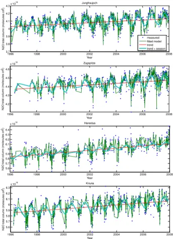
5.3 N2O trends
The fitted N2O models are presented in Fig. 4 and the es-timated trends are listed in Table 5. The N2O trends vary from approximately 0.2±0.01 % yr−1 at Jungfraujoch and Zugspitze to 0.29±0.02 and 0.4±0.02 % yr−1 at the two stations located further north. Earlier IPCC (2007) has re-ported a N2O trend for the last decade of 0.26 % yr−1. This trend is verified by in situ measurements by Haszpra et al. (2008) and total columns by Rinsland et al. (2009) who both report trends of 0.25±0.003 % yr−1. The estimated N2O trends for Jungfraujoch and Zugspitze are a bit weaker than the earlier reported trends but in close agreement to each other. The trends for Kiruna and especially Harestua are stronger than the reported trends and are not in agree-ment with each other. This trend discrepancy is unexpected since N2O is well mixed in the atmosphere due to its tro-pospheric lifetime of 114 years (Davidson, 2009). To ex-clude that instrumental errors are the cause for the deviating N2O trends we have estimated total column trends also for CO2 from Harestua and Kiruna. CO2was used because its atmospheric circulation time is similar to the lifetime N2O and that both of the species are measured with the same type of detector (InSb detector). The CO2 retrieval was conducted in the 2620-2630 cm−1region with Hitran08 line parameters (R. Kohlhepp and F. Hase, private communica-tion, 2010). The estimated CO2trends for the two stations showed to be very similar, 0.50±0.06 % yr−1 for Harestua and 0.56±0.04 % yr−1for Kiruna on a 2-σ basis and this corresponds well to the in situ trend of roughly 0.51 % pre-sented by IPCC (2007) (the trend is based on an increase of 19 ppm from 1995 to 2005). From this test it is concluded that the FTIR instruments at Harestua and Kiruna behaved well during the studied period.
To further investigate the trend discrepancy between the FTIR stations trends we derived tropospheric- and strato-spheric partial columns from the FTIR data at each sta-tion. The partial columns was derived with a weight func-tion described by Gardiner et al. (2008) which use the aver-age tropopause height and its standard deviation, here taken from the ECMWF model. The trends in the partial columns were estimated with a function consisting of a linear trend and a seasonal cycle with a phase. All the estimated tro-pospheric trends were in the range of 0.19±0.01 % yr−1
1996 1998 2000 2002 2004 2006 2008
3.7 3.8 3.9 4 4.1 4.2 4.3x 10
18
Year
N
2
O
t
o
ta
l
co
lu
m
n
(
m
o
le
cu
le
s
cm
-2)
Jungfraujoch
measured fitted model trend trend + season
1996 1998 2000 2002 2004 2006 2008
4.2 4.3 4.4 4.5 4.6
x 1018 Zugspitze
Year
N
2
O
t
o
ta
l
co
lu
m
n
(
m
o
le
cu
le
s
cm
-2)
1996 1998 2000 2002 2004 2006 2008
5.6 5.7 5.8 5.9 6 6.1 6.2 6.3 6.4
x 1018 Harestua
Year
N
2
O
t
o
ta
l
co
lu
m
n
(
m
o
le
cu
le
s
cm
-2)
1996 1998 2000 2002 2004 2006 2008
5.6 5.7 5.8 5.9 6 6.1 6.2 6.3
x 1018 Kiruna
Year
N
2
O
t
o
ta
l
co
lu
m
n
(
m
o
le
cu
le
s
cm
-2)
Fig. 4.As Fig. 3a but for N2O total columns.
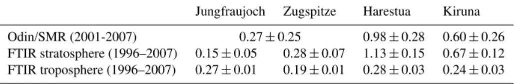
to 0.28±0.03 % yr−1while the stratospheric trends showed large inter station variability with strong positive trends at Harestua and Kiruna and weak positive trends at Jungfrau-joch and Zugspitze, Table 6. Earlier, Gardiner et al. (2008) also showed this behaviour.
Table 6.Stratospheric N2O trends from SMR and FTIR data presented in % yr−1. The trends are presented with associated 2-σconfidence
intervals and use the 2005 average partial column as reference.
Jungfraujoch Zugspitze Harestua Kiruna Odin/SMR (2001-2007) 0.27±0.25 0.98±0.28 0.60±0.26 FTIR stratosphere (1996–2007) 0.15±0.05 0.28±0.07 1.13±0.15 0.67±0.12 FTIR troposphere (1996–2007) 0.27±0.01 0.19±0.01 0.28±0.03 0.24±0.03
20014 2002 2003 2004 2005 2006 2007 2008
5 6 7 8 9 10x 10
17
Year
N
2
O
p
a
rt
ia
l
co
lu
m
n
(
m
o
l
cm
-2)
Odin/SMR Jungfraujoch
measured fitted model linear trend
20013 2002 2003 2004 2005 2006 2007 2008
4 5 6 7 8x 10
17
N
2
O
p
a
rt
ia
l
co
lu
m
n
(
m
o
l
cm
-2)
Year Odin/SMR Kiruna
19967 1998 2000 2002 2004 2006 2008
8 9 10 11 12x 10
17
N
2
O
p
a
rt
ia
l
co
lu
m
n
(
m
o
l
cm
-2)
Year FTIR Jungfraujoch
19961 1998 2000 2002 2004 2006 2008
2 3 4 5 6 7x 10
17
N
2
O
p
a
rt
ia
l
co
lu
m
n
(
m
o
l
cm
-2)
Year FTIR Kiruna
Fig. 5.Stratospheric partial columns of N2O with fitted seasonal function and linear trend for Jungfraujoch and Kiruna from the SMR instrument onboard the Odin satellite and solar FTIR data.
at Harestua. A slightly weaker trend is seen in Kiruna and a much weaker trend is estimated in the Alp region. It hence seems that the difference in total column trends between the Alp region and Harestua and Kiruna is caused by the differ-ences in the stratospheric column trends and it appears that the highest trend is found at the vortex edge, above Harestua as observed by FTIR and the SMR onboard Odin. We do not have an explanation for this behaviour but is likely related to the atmospheric circulation, since N2O has a very long lifetime which would smooth out differences in sources and sinks.
5.4 Model stability
To obtain the confidence intervals, the residual from the model is assumed to be normally distributed with constant variance around a mean value of zero and to be free from au-tocorrelation. The residual distributions from the regression models for all FTIR stations are shown in the lower left panel in Fig. 6 (for CH4)and in Fig. 7 (for N2O), also presented is a normal distribution based on the standard deviation from each of the residuals. These distributions indicate that the assumption of normal distribution is justified. In the lower right panels in Figs. 6 and 7 the residuals are plotted as a function of the fitted model. To justify the constant variance assumption the residuals are expected to be randomly scat-tered around a constant level of zero. In our case we conclude that this assumption is justified for all the regression mod-els. Also, to verify the assumption that no autocorrelation is present in the time series we look at the residual as a func-tion of time, this can be seen in the upper panel in Figs. 6 and 7. Shapes such as cycles might indicate autocorrelation and may make the confidence intervals for the estimated trends larger. Based on the residual analysis we conclude that no strong autocorrelation is presented in any of the regression models.
When working with multiple regression models, one al-ways needs to consider multicolinearity. Multicolinearity is when one or several of the independent variables in the re-gression model contain similar information, i.e. are linearly dependent. The presence of multicolinearity may result in physically unrealistic values or signs and large confidence intervals of the estimated regression coefficients. To investi-gate the presence of multicolinearity in the regression model the concept of the variance inflation factor, VIF factor, is used (Neter et al., 1990). A VIF factor of 1 indicates totally independent variables and a factor larger than 10 indicates serious multicolinearity in the model (Neter et al., 1990). In our case the calculated VIF factors are well below 10 for all FTIR stations and both of the species under investigation.
To verify that the 1 % criteria, earlier defined in Sect. 4.4, in the calculations of the anomalies is appropriate a sensi-tivity analysis is performed on all the regression models. In the analysis the estimated linear trend and the adjustedR2
1996 1998 2000 2002 2004 2006 2008 2010 -2
-1.5 -1 -0.5 0 0.5 1 1.5
2x 10
18
Year
C
H
4
r
e
si
d
u
a
l
(m
o
le
cu
le
s
cm
-2)
Jungfraujoch
-4 -3 -2 -1 0 1 2 3
x 1017 0
50 100 150 200
CH4 residual (molecules cm-2)
N
u
m
b
e
r
2.2 2.25 2.3 2.35 2.4 2.45
x 1019 -6
-4 -2 0 2 4x 10
17
Fitted model (molecules cm-2)
C
H
4
r
e
si
d
u
a
l
(m
o
le
cu
le
s
cm
-2)
1996 1998 2000 2002 2004 2006 2008 2010
-2 -1.5 -1 -0.5 0 0.5 1 1.5
2x 10
18
Year
C
H
4
r
e
si
d
u
a
l
(m
o
le
cu
le
s
cm
-2)
Zugspitze
-1 -0.5 0 0.5 1
x 1018 0
50 100 150 200 250 300
CH4 residual (molecules cm-2)
N
u
m
b
e
r
2.4 2.45 2.5 2.55 2.6 2.65
x 1019 -1.5
-1 -0.5 0 0.5 1 1.5x 10
18
Fitted model (molecules cm-2)
C
H
4
r
e
si
d
u
a
l
(m
o
le
cu
le
s
cm
-2)
Fig. 6.CH4residuals and distributions of the Jungfraujoch and Zugspitze FTIR time series when a piecewise linear trend is used.
the parameter is changed. The change of the linear trend in the total columns of CH4and N2O is largest when increasing from polynomial order zero to a first order and to a second order polynomial for the total column of HF (0, 1, 2) while for the other parameters the change is largest from zero to first (0,1). At higher order of polynomial only very small changes in the estimated trends are observed. It can also be seen that the adjustedR2value not increase for polynomials with higher order than two for HF and one for the other pa-rameters. From the sensitivity analysis we conclude that the 1 % criterion is appropriate for deriving the anomalies.
5.5 Method comparison
The results of the multiple regression model has been com-pared to two other trend methods. The first method,
1996 1998 2000 2002 2004 2006 2008 2010 -2
-1.5 -1 -0.5 0 0.5 1 1.5
2x 10
18
Year
C
H
4
r
e
si
d
u
a
l
(m
o
le
cu
le
s
cm
-2)
Harestua
-2 -1.5 -1 -0.5 0 0.5 1 1.5 x 10¹⁸ 0
20 40 60 80 100 120 140
CH4 residual (molecules cm-2)
N
u
m
b
e
r
3.2 3.3 3.4 3.5 3.6 3.7 x 10¹⁹ -3
-2 -1 0 1 2x 10
18
Fitted model (molecules cm-2)
C
H
4
r
e
si
d
u
a
l
(m
o
le
cu
le
s
cm
-2)
1996 1998 2000 2002 2004 2006 2008 2010
-2 -1.5 -1 -0.5 0 0.5 1 1.5
2x 10
18
Year
C
H
4
r
e
si
d
u
a
l
(m
o
le
cu
le
s
cm
-2)
Kiruna
-10 -5 0 5
x 1017 0
50 100 150
CH4 residual (molecules cm-2)
N
u
m
b
e
r
3.2 3.3 3.4 3.5 3.6 3.7 x 10¹⁹ -1.5
-1 -0.5 0 0.5
1x 10
18
Fitted model (molecules cm-2)
C
H
4
r
e
si
d
u
a
l
(m
o
le
cu
le
s
cm
-2)
Fig. 6.Continued.
the multiple regression model, the Bootstrap algorithm and by the simple least squares fit of a straight line and a sea-sonal component, for the 1996–2009 and 1996–2007 period for CH4and N2O total columns respectively. The outcome of the study is presented in Table 7 which shows the estimated trends with associated 95 % confidence limits. The three trend methods show all results that are in relatively close agreement to each other. In general, the multiple regres-sion method has slightly smaller confidence intervals than the other two methods. The trends obtained from the Boot-strap algorithm and the model with a linear trend and
1996 1998 2000 2002 2004 2006 2008 -2.5
-2 -1.5 -1 -0.5 0 0.5 1 1.5x 10
17
Year
N
2
O
r
e
si
d
u
a
l
(m
o
le
cu
le
s
cm
-2)
Jungfraujoch
-8 -6 -4 -2 0 2 4 6 x 10¹⁶ 0
50 100 150
N2O residual (molecules cm-2)
N
u
m
b
e
r
3.7 3.8 3.9 4 4.1 4.2 4.3 x 10¹⁸ -1
-0.5 0 0.5
1x 10
17
Fitted model (molecules cm-2)
N
2
O
r
e
si
d
u
a
l
(m
o
le
cu
le
s
cm
-2)
1996 1998 2000 2002 2004 2006 2008
-2.5 -2 -1.5 -1 -0.5 0 0.5 1 1.5x 10
17
Year
N
2
O
r
e
si
d
u
a
l
(m
o
le
cu
le
s
cm
-2)
Zugspitze
-2 -1.5 -1 -0.5 0 0.5 1 x 10¹⁷ 0
50 100 150 200 250
N2O residual (molecules cm-2)
N
u
m
b
e
r
4.1 4.2 4.3 4.4 4.5 4.6 4.7 x 10¹⁸ -2.5
-2 -1.5 -1 -0.5 0 0.5 1 1.5x 10
17
Fitted model (molecules cm-2)
N
2
O
r
e
si
d
u
a
l
(m
o
le
cu
le
s
cm
-2)
Fig. 7.N2O residuals and distributions of the Jungfraujoch and Zugspitze FTIR time series.
time series the estimated trend values will have an impact on the final trend result and potentially make the confidence intervals wider.
The trends estimated from the multiple regression method differ in magnitude with up to 31 % and have an uncertainty that differs up to 300 % compared to the other two methods. This difference is most likely because the multiple regres-sion model takes the atmospheric variability into account and hence reduces the unexplained part of the trend model. From the method comparison and model stability analysis we
con-clude that the multiple regression model gives the most re-liable trends since it takes the atmospheric variability into account and fulfils the statistical assumptions presented in Sect. 5.4.
6 Discussion and conclusion
1996 1998 2000 2002 2004 2006 2008 -2.5
-2 -1.5 -1 -0.5 0 0.5 1 1.5x 10
17
Year
N
2
O
r
e
si
d
u
a
l
(m
o
le
cu
le
s
cm
-2)
Harestua
-3 -2 -1 0 1 2 3
x 1017 0
20 40 60 80 100 120 140
N2O residual (molecules cm-2)
N
u
m
b
e
r
5.4 5.6 5.8 6 6.2 6.4 x 10¹⁸ -4
-3 -2 -1 0 1 2 3 4x 10
17
Fitted model (molecules cm-2)
N
2
O
r
e
si
d
u
a
l
(m
o
le
cu
le
s
cm
-2)
1996 1998 2000 2002 2004 2006 2008
-2.5 -2 -1.5 -1 -0.5 0 0.5 1 1.5x 10
17
Year
N
2
O
r
e
si
d
u
a
l
(m
o
le
cu
le
s
cm
-2)
Kiruna
-4 -3 -2 -1 0 1 2 3 x 10¹⁷ 0
50 100 150 200 250
N2O residual (molecules cm-2)
N
u
m
b
e
r
5.4 5.6 5.8 6 6.2 6.4 x 10¹⁸ -6
-4 -2 0 2 4x 10
17
Fitted model (molecules cm-2)
N
2
O
r
e
si
d
u
a
l
(m
o
le
cu
le
s
cm
-2)
Fig. 7.Continued.
trends for both species at the northern sites and weaker trends at the Alpine stations.
When it comes to CH4this latitudinal difference is not sur-prising since the atmospheric concentration of the species are highly influenced by local sources. At high latitudes wetland contributes up to 25 % of the CH4total emissions and these wetlands have shown to be sensitive to climate change (Jackowicz-Korczynski et al., 2010). In addition Russian natural gas is produced at the same latitudes as Harestua and Kiruna. These might be two possible
rea-sons for the stronger trends detected at the northern latitude sites (Harestua and Kiruna) compared to the two Alpine sta-tions.
sta-Table 7. Estimated linear trends from the total columns of CH4and N2O. The trends are presented in percent per year (% yr−1)with the
reference year given as the average value of year 2000. All trends are given with associated 95σconfidence limits.
Trend model Species Jungfraujoch Zugspitze Harestua Kiruna Multiple regression model CH4 0.16±0.01 0.13±0.01 0.25±0.02 0.21±0.01
N2O 0.21±0.01 0.19±0.01 0.40±0.02 0.29±0.02
Bootstrap algorithm CH4 0.16±0.02 0.09±0.03 0.28±0.04 0.26±0.04 N2O 0.25±0.03 0.22±0.03 0.45±0.06 0.33±0.05
Linear trend with CH4 0.16±0.01 0.09±0.02 0.28±0.03 0.26±0.02 seasonal component N2O 0.25±0.02 0.22±0.02 0.46±0.04 0.34±0.03
tions. One possible explanation could be the strengthen-ing of the Brewer Dobson circulation as described by Li et al. (2010). This circulation transports air masses from the tropical tropopause into the stratosphere and towards the poles. If the circulation gets stronger with time more N2O is transported towards Harestua and Kiruna with a stratospheric trend as result. The stations located further south are less in-fluenced by this transport and hence a weaker stratospheric trend is detected. Another possible reason to the trend differ-ences could be a trend in the tropopause height due to climate change or other changes in the atmospheric dynamics. Lin-ear trends were therefore estimated from the tropopause data, the earlier used ECMWF data, for the FTIR stations. All the estimated trends were close to zero and insignificant. From this we conclude that a change in the tropopause altitude is most likely not responsible for the stratospheric N2O trends. We conclude that more studies are needed regarding the lati-tudinal difference in stratospheric N2O.
Acknowledgements. This paper is funded by the EU project
HYMN. The author would like to thank Anders Strandberg and Glenn Persson for Harestua FTIR measurement and Marston John-ston for ECMWF data. P. Duchatelet and E. Mahieu have further been supported by the Belgian Federal Science Policy Office (BEL-SPO, Brussels). The International Foundation High Altitude Research Stations Jungfraujoch and Gornergrat (HFSJG, Bern) is also acknowledged. T. Blumenstock, F. Hase and M. Schneider would like to thank the Institute of Space Physics (IRF) Kiruna and in particular Uwe Raffalski (IRF) for supporting the measurements at Kiruna. Odin is a Swedish-led satellite project funded jointly by the Swedish National Space Board (SNSB), the Canadian Space Agency (CSA), the Centre National d’Etudes Spatiales (CNES) in France and the National Technology Agency of Finland (Tekes). The Odin mission is since 2007 supported through the 3rd party mission programme of the European Space Agency (ESA). Edited by: C. Gerbig
References
Bates, D. R. and Hays, P. B.: Atmospheric Nitrous Oxide, Planet. Space Sci., 15, 189–197, 1967.
Davidson, E. A.: The contribution of manure and fertilizer nitrogen to atmospheric nitrous oxide since 1860, Nat. Geosci., 2, 659– 662, doi:10.1038/Ngeo608, 2009.
DeMazi`ere, M., Vigouroux, C., Gardiner, T., Coleman, M., Woods, P., Ellingsen, K., Gauss, M., Isaksen, I., Blumenstock, T., Hase, F., Kramer, I., Camy-peyret, C., Chelin, P., Mahieu, E., De-moulin, P., Duchatelet, P., Mellqvist, J., Strandberg, A., Velazco, V., Notholt, J., Sussmann, R., Stremme, W., and Rockmann, A.: The exploitation of ground-based Fourier transform infrared ob-servations for the evaluation of tropospheric trends of greenhouse gases over Europe, Environm. Sci., 2, 283–293, 2005.
Dlugokencky, E. J., Steele, L. P., Lang, P. M., and Masarie, K. A.: The Growth-Rate and Distribution of Atmospheric Methane, J. Geophys. Res.-Atmos., 99, 17021–17043, 1994.
Dlugokencky, E. J., Houweling, S., Bruhwiler, L., Masarie, K. A., Lang, P. M., Miller, J. B., and Tans, P. P.: Atmospheric methane levels off: Temporary pause or a new steady-state?, Geophys. Res. Lett., 30, 1992, doi:10.1029/2003gl018126, 2003. Dlugokencky, E. J., Bruhwiler, L., White, J. W. C., Emmons, L.
K., Novelli, P. C., Montzka, S. A., Masarie, K. A., Lang, P. M., Crotwell, A. M., Miller, J. B., and Gatti, L. V.: Observational constraints on recent increases in the atmospheric CH4burden, Geophys. Res. Lett., 36, L18803, doi:10.1029/2009gl039780, 2009.
Efron, B. and Tibshirani, R.: An introduction to the bootstrap, Monographs on statistics and applied probability, 57, Chapman & Hall, New York, USA, xvi, 436 pp., 1993.
Gardiner, T., Forbes, A., de Mazie`re, M., Vigouroux, C., Mahieu, E., Demoulin, P., Velazco, V., Notholt, J., Blumenstock, T., Hase, F., Kramer, I., Sussmann, R., Stremme, W., Mellqvist, J., Strand-berg, A., Ellingsen, K., and Gauss, M.: Trend analysis of green-house gases over Europe measured by a network of ground-based remote FTIR instruments, Atmos. Chem. Phys., 8, 6719–6727, doi:10.5194/acp-8-6719-2008, 2008.
Hase, F., Blumenstock, T., and Paton-Walsh, C.: Analysis of the instrumental line shape of high-resolution Fourier transform IR spectrometers with gas cell measurements and new retrieval soft-ware, Appl. Optics, 38, 3417–3422, 1999.
M., Jones, N. B., Rinsland, C. P., and Wood, S. W.: Intercompar-ison of retrieval codes used for the analysis of high-resolution, ground-based FTIR measurements, J. Quant. Spectrosc. Ra., 87, 25–52, doi:10.1016/j.jqsrt.2003.12.008, 2004.
Haszpra, L., Barcza, Z., Hidy, D., Szilagyi, I., Dlugokencky, E., and Tans, R.: Trends and temporal variations of major green-house gases at a rural site in Central Europe, Atmos. Environ., 42, 8707–8716, doi:10.1016/j.atmosenv.2008.09.012, 2008. IPCC: Contribution of Working Group I to the Fourth Assessment
Report of the Intergovernmental Panel on Climate Change, 2007, Cambridge University Press, Cambridge, United Kingdom and New York, NY, USA, 2007.
Jackowicz-Korczynski, M., Christensen, T. R., Backstrand, K., Crill, P., Friborg, T., Mastepanov, M., and Strom, L.: Annual cy-cle of methane emission from a subarctic peatland, J. Geophys. Res.-Biogeo., 115, G02009, doi:10.1029/2008jg000913, 2010. Jones, A., Urban, J., Murtagh, D. P., Eriksson, P., Brohede, S.,
Ha-ley, C., Degenstein, D., Bourassa, A., von Savigny, C., Sonkaew, T., Rozanov, A., Bovensmann, H., and Burrows, J.: Evolu-tion of stratospheric ozone and water vapour time series studied with satellite measurements, Atmos. Chem. Phys., 9, 6055–6075, doi:10.5194/acp-9-6055-2009, 2009.
Li, F., Newman, P. A., and Stolarski, R. S.: Relationships be-tween the Brewer-Dobson circulation and the southern annu-lar mode during austral summer in coupled chemistry-climate model simulations, J. Geophys. Res.-Atmos., 115, D15106, doi:10.1029/2009jd012876, 2010.
Mellqvist, J., Galle, B., Blumenstock, T., Hase, F., Yashcov, D., Notholt, J., Sen, B., Blavier, J.-F., Toon, G. C., and Chip-perfield, M. P.: Ground-Based FTIR observations of chlorine activation and ozone depletion inside the Arctic vortex dur-ing the winter of 1999/2000, J. Geophys. Res., 107, 8263, doi:10.1029/2001JD001080, 2002.
Montgomery, D. C., Jennings, C. L., and Kulahci, M.: Introduc-tion to time series analysis and forecasting, in: Wiley series in probability and statistics, edited by: Hoboken, N. J., Wiley-Interscience, xi, 445 pp., 2008.
Murtagh, D., Frisk, U., Merino, F., Ridal, M., Jonsson, A., Stegman, J., Witt, G., Eriksson, P., Jimenez, C., Megie, G., de la Noe, J., Ricaud, P., Baron, P., Pardo, J. R., Hauchcorne, A., Llewellyn, E. J., Degenstein, D. A., Gattinger, R. L., Lloyd, N. D., Evans, W. F. J., McDade, I. C., Haley, C. S., Sioris, C., von Savigny, C., Solheim, B. H., McConnell, J. C., Strong, K., Richardson, E. H., Leppelmeier, G. W., Kyrola, E., Auvinen, H., and Oikarinen, L.: An overview of the Odin atmospheric mission, Can. J. Phys., 80, 309–319, doi:10.1139/P01-157, 2002.
Neter, J., Wasserman, W., and Kutner, M. H.: Applied linear statis-tical models : regression, analysis of variance, and experimental designs, 3rd edn., Irwin, Homewood, IL, xvi, 1181 pp., 1990. Rinsland, C. P., Jones, N. B., Connor, B. J., Logan, J. A.,
Pougatchev, N. S., Goldman, A., Murcray, F. J., Stephen, T. M., Pine, A. S., Zander, R., Mahieu, E., and Demoulin, P.: Northern and southern hemisphere ground-based infrared spectroscopic measurements of tropospheric carbon monoxide and ethane, J. Geophys. Res.-Atmos., 103, 28197–28217, 1998.
Rinsland, C. P., Chiou, L., Boone, C., Bernath, P., Mahieu, E., and Zander, R.: Trend of lower stratospheric methane (CH4) from atmospheric chemistry experiment (ACE) and atmospheric trace molecule spectroscopy (ATMOS) measurements, J. Quant.
Spec-trosc. Ra., 110, 1066–1071, doi:10.1016/j.jqsrt.2009.03.024, 2009.
Rodgers, C. D.: Inverse Methods for Atmospheric Sounding, Series on Atmospheric, Oceanic and Planetary Physics, 2, 55–63, 2000. Simpson, I. J., Rowland, F. S., Meinardi, S., and Blake, D. R.: In-fluence of biomass burning during recent fluctuations in the slow growth of global tropospheric methane, Geophys. Res. Lett., 33, L22808, doi:10.1029/2006gl027330, 2006.
Strong, K., Wolff, M. A., Kerzenmacher, T. E., Walker, K. A., Bernath, P. F., Blumenstock, T., Boone, C., Catoire, V., Cof-fey, M., De Mazire, M., Demoulin, P., Duchatelet, P., Dupuy, E., Hannigan, J., Hpfner, M., Glatthor, N., Griffith, D. W. T., Jin, J. J., Jones, N., Jucks, K., Kuellmann, H., Kuttippurath, J., Lam-bert, A., Mahieu, E., McConnell, J. C., Mellqvist, J., Mikuteit, S., Murtagh, D. P., Notholt, J., Piccolo, C., Raspollini, P., Ri-dolfi, M., Robert, C., Schneider, M., Schrems, O., Semeniuk, K., Senten, C., Stiller, G. P., Strandberg, A., Taylor, J., Te´tard, C., Toohey, M., Urban, J., Warneke, T., and Wood, S.: Validation of ACE-FTS N2O measurements, Atmos. Chem. Phys., 8, 4759– 4786, doi:10.5194/acp-8-4759-2008, 2008.
Sussmann, R. and Borsdorff, T.: Technical Note: Interference errors in infrared remote sounding of the atmosphere, Atmos. Chem. Phys., 7, 3537–3557, doi:10.5194/acp-7-3537-2007, 2007. Sussmann, R., Stremme, W., Buchwitz, M., and de Beek, R.:
Val-idation of ENVISAT/SCIAMACHY columnar methane by solar FTIR spectrometry at the Ground-Truthing Station Zugspitze, Atmos. Chem. Phys., 5, 2419–2429, doi:10.5194/acp-5-2419-2005, 2005.
Tiao, G. C., Reinsel, G. C., Xu, D. M., Pedrick, J. H., Zhu, X. D., Miller, A. J., Deluisi, J. J., Mateer, C. L., and Wuebbles, D. J.: Effects of Autocorrelation and Temporal Sampling Schemes on Estimates of Trend and Spatial Correlation, J. Geophys. Res.-Atmos., 95, 20507–20517, 1990.
Toon, G. C., Blavier, J.-F., Sen, B., Salawitch, R. J., G. B. Osterman, Notholt, J., Rex, M., McElroy, C. T., and Russell, J. M.: Ground-based observations of Arctic O3 loss during spring and summer 1997, J. Geophys. Res., 104, 497–510, 1997.
Twomey, S.: Introduction to the mathematics of inversion in remote sensing and indirect measurements, Dover Publications, Mine-ola, N.Y., x, 237 pp., 1996.
Urban, J., Lautie, N., Le Flochmoen, E., Jimenez, C., Eriksson, P., de La Noe, J., Dupuy, E., Ekstrom, M., El Amraoui, L., Frisk, U., Murtagh, D., Olberg, M., and Ricaud, P.: Odin/SMR limb obser-vations of stratospheric trace gases: Level 2 processing of ClO, N2O, HNO3, and O-3, J. Geophys. Res.-Atmos., 110, D14307,
doi:10.1029/2004jd005741, 2005a.
Urban, J., Lautie, N., Le Flochmoen, E., Jimenez, C., Eriksson, P., de La Noe, J., Dupuy, E., El Amraoui, L., Frisk, U., Jegou, F., Murtagh, D., Olberg, M., Ricaud, P., Camy-Peyret, C., Du-four, G., Payan, S., Huret, N., Pirre, M., Robinson, A. D., Har-ris, N. R. P., Bremer, H., Kleinbohl, A., Kullmann, K., Kunzi, K., Kuttippurath, J., Ejiri, M. K., Nakajima, H., Sasano, Y., Sugita, W., Yokota, T., Piccolo, C., Raspollini, P., and Ridolfi, M.: Odin/SMR limb observations of stratospheric trace gases: Validation of N2O, J. Geophys. Res.-Atmos., 110, D09301,
doi:10.1029/2004jd005394, 2005b.
Observations of Trace Gases in the Polar Lower Stratosphere during 2004–2005, Proc. ESA First Atmospheric Science Con-ference, edited by: Lacoste, H., ESA-SP-628, ISBN-92-9092-939-1, 2006.
Weatherhead, E. C., Reinsel, G. C., Tiao, G. C., Meng, X. L., Choi, D. S., Cheang, W. K., Keller, T., DeLuisi, J., Wuebbles, D. J., Kerr, J. B., Miller, A. J., Oltmans, S. J., and Frederick, J. E.: Factors affecting the detection of trends: Statistical considera-tions and applicaconsidera-tions to environmental data, J. Geophys. Res.-Atmos., 103, 17149–17161, 1998.
Vigouroux, C., De Mazie`re, M., Demoulin, P., Servais, C., Hase, F., Blumenstock, T., Kramer, I., Schneider, M., Mellqvist, J., Strandberg, A., Velazco, V., Notholt, J., Sussmann, R., Stremme, W., Rockmann, A., Gardiner, T., Coleman, M., and Woods, P.: Evaluation of tropospheric and stratospheric ozone trends over Western Europe from ground-based FTIR network observations, Atmos. Chem. Phys., 8, 6865–6886, doi:10.5194/acp-8-6865-2008, 2008.
Yurganov, L. N., Blumenstock, T., Grechko, E. I., Hase, F., Hyer, E. J., Kasischke, E. S., Koike, M., Kondo, Y., Kramer, I., Le-ung, F. Y., Mahieu, E., Mellqvist, J., Notholt, J., Novelli, P. C., Rinsland, C. P., Scheel, H. E., Schulz, A., Strandberg, A., Suss-mann, R., Tanimoto, H., Velazco, V., Zander, R., and Zhao, Y.: A quantitative assessment of the 1998 carbon monoxide emission anomaly in the Northern Hemisphere based on total column and surface concentration measurements, J. Geophys. Res.-Atmos., 109, D15305, doi:10.1029/2004jd004559, 2004.