Abstract— In this paper, a software for design and analysis of
frequency selective surfaces (FSS) based on the equivalent circuit model is presented, with emphasis on teaching students in the interaction between FSS parameters. Tools to design FSSs and a tutorial with theoretical elements of the equivalent circuit method, applied to FSS, compose this software. The software can be used at FSS analysis and design course to consolidate the first theoretical and illustrated concepts.
Index Terms — Frequency selective surfaces, equivalent circuit method, interactive computing, simulation software.
I. INTRODUCTION
Since the invention of the electronic computer there are two divergent opinions to show how this
device should be used. One group saw the computer’s principal use as a number manipulator: an
extensive, ultrafast, and accurate calculator. A second group envisioned the computer as a symbol
manipulator that might be taught to use logic and make decisions in a human fashion [1].
Frequency selective surfaces (FSS) are periodic structures in two dimensions that can provide
frequency filtering to incoming electromagnetic waves. Traditional FSS structures have been
investigated over the years for a variety of applications (e.g., frequency filters or diplexers in high
performance reflector antenna systems, advanced radome designs, and smart surfaces for stealth
applications) [2].
The analysis and design of FSS, and the calculation of their parameters, is inherently
multidisciplinary, demanding knowledge of antenna, electromagnetic theory and FSS analysis and
design disciplines. For example, when a parameter is modified in a FSS, this modification has some
electromagnetic consequences, and hence also affects the frequency filtering.
In recent years, a number of electromagnetic simulation commercial software have appeared on the
market, such as CST Microwave Studio®, Ansoft Designer®, and Ansoft HFSS®, and also a number of
A periodic array consisting of conducting patch or aperture elements is known as a frequency
selective surface (FSS), or dichroic. FSS may have low-pass or high-pass spectral behavior,
depending on the array element type (i.e., patch or aperture), similarly to the frequency filters in
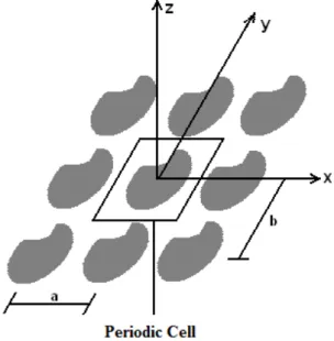
traditional radio-frequency (RF) [10]. A Two-dimensional planar periodic structure is shown in Fig. 1.
Fig. 1. Geometry of a two-dimensional periodic structure.
Many design parameters and principles are associated with the periodic structure, such as element
shape, size, lattice geometry, dielectrics, grating lobes, and Wood’s anomaly. Some of the most
common element shapes are: circular, rectangular, dipole, cross dipole, Jerusalem cross, tripole, three-
or four-legged dipole, ring, square loop and gridded square loop [10]. There are element formats that
can be obtained from a combination or modification of simple elements such as those mentioned
above, and elements of very complex shapes such as convolutional or fractals [11-13].
An FSS is a periodic array of aperture or patch elements, which are shown in Fig. 2.
Aperture-element FSS reflects at low frequencies and transmits at high frequencies (similar to a high-pass
filter), whereas the patch-element FSS transmits at low frequencies and reflects at high frequencies
(similar to a low-pass filter) [11].
Several methods have been used to analyze FSS. One of the simplest methods is the equivalent
circuit model [14, 15]. In this analysis the various strip elements that form a freestanding patch
element in a periodic array are modeled as inductive and capacitive components on a transmission
line. From the solution of this circuit, the reflection and transmission coefficients of the FSS are
(a) (b)
Fig. 2. FSS elements: (a) type aperture and (b) type patch.
III. SOFTWARE DESCRIPTION
The simulation software will be presented with an emphasis on the pedagogical point of view. The
software is programmed in MATLAB®, which uses its own language sometimes called M-code or
simply M, to facilitate both numerical calculations and graphical representations. The program
analyzes an FSS mounted on a dielectric isotropic layer.
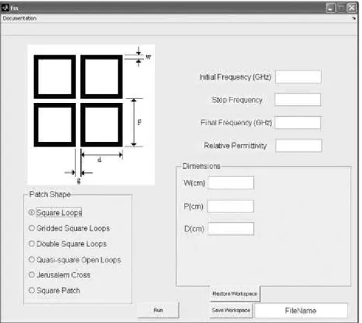
The graphical interface is a key point in this program. When the program is initiated, a selection
menu displays the six possible FSS designs: square loops, gridded square loops, double square loops,
quasi-square open loops, Jerusalem cross and square patch. Fig. 3 shows the main screen program.
The elements of the main design screen are:
• Tool bar; • Patch Shape; • Picture; • Dimensions;
• Selecting Frequency Parameters; • Run Button;
• Save and Restore Workspace Buttons.
In the upper side of the main screen, the tool bar shows menu button for documentation, when the
user click in this button will appear the menu shown in Fig. 4. Chosen one of the structures, a pdf file
is opened and the principal proprieties, equivalent circuit and mathematical model are presented.
The element Patch Shape comprises six options for element shapes to create the FSS. Each shape
takes a different set of physical parameters and image for each of the options. Fig. 5 shows this item.
Fig. 3. Complete layout of the FSS simulation software.
Fig. 4. Additional Information about each shape.
Fig. 6. Picture showing the physical parameters of the chosen geometry.
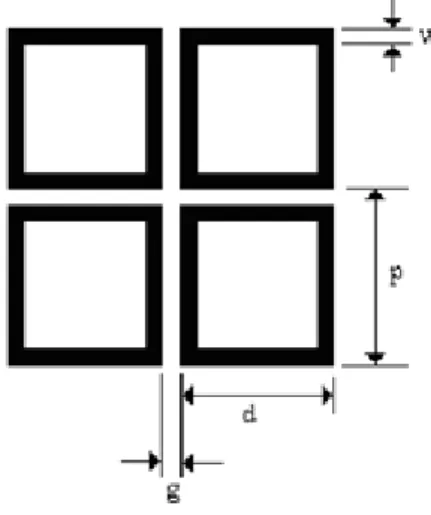
Dimensions comprise the set of variables or parameters required to do the analysis of the structure,
these parameters are shown in the Picture item. For the option of square loop you can view the
parameters shown in Fig. 7.
Fig. 7. Selecting physical parameters.
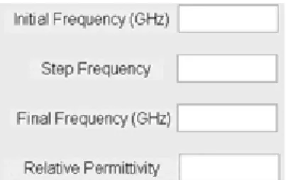
The element Frequency Parameters shows fields where frequency domain parameters and the relative permittivity of the substrate are placed. The user can take more information about each shape
by menu Documentation, where the principal proprieties, equivalent circuit and mathematical model
are presented. Fig. 8 shows this field.
When the user click on the button Run Button, the software analysis begins, one window with the
S21 response of structure is plotted when the analysis finished.
The shape, parameters and results can be saved and restored anytime placing the file name and click
Fig. 8. Selecting frequency domain parameters and substrate relative permittivity.
IV. CIRCUIT EQUIVALENT METHOD
As mentioned earlier, the simulation software uses as analysis method the equivalent circuit model.
This technique requires very limited computational resources when compared to full wave analysis
methods, so it is useful to quickly predict the performance of that structures. The model also provides
a useful physical view on how the FSS operates when its parameters are changed.
The starting point for the development of equivalent circuits for FSS structures is the representation
of an infinite array of parallel conducting strips, developed by Marcuvitz [16]. The metal strips have
zero thickness, a width, w, and periodicity, p. The plane wave illuminates the strips with an angle φ.
The inductive equivalent reactance is given as [16]:
(
)
(
)
0 2
L
X p co s w
F p,w, , ln cos ec G p,w, ,
Z p
φ π
λ φ λ φ
λ = = +
(1)
where,
(
)
(
)
(
)
(
)
2 2 2 22 2 4
2 6
0 5 1 1 4
4
1 1 2
4 2 8
, C C C C
G p,w, ,
C C C C
β
β β
λ φ
β β β
β β + − + − + − + − − − + + = − + + − + + (2) 2 1 1 2 1 C
p sinφ p cosφ
λ λ ± = − ± − (3) 2 w sin p π β =
(4)
and λ is the wavelength.
At the same way, the incident magnetic field vector is parallel to the metal strips and it illuminates
the array with an angle θ. The strips have periodicity, p, and a gap between the strips, g. The
capacitive susceptance is calculated by [16]:
(
)
(
)
0 4 4 2 CB p co s w
F p,w, , ln cos ec G p,w, ,
Z p
θ π
λ θ λ θ
λ = = +
(5)
The function
G p,g , ,
(
λ θ
)
can be solved by (1), Just change φ by θ and w by g.Equations (1) to (5) are appropriated to wavelengths and incidence angles between the range:
(
1)
1The method has some limitations, since it is generally useful only for normal incidence of plane
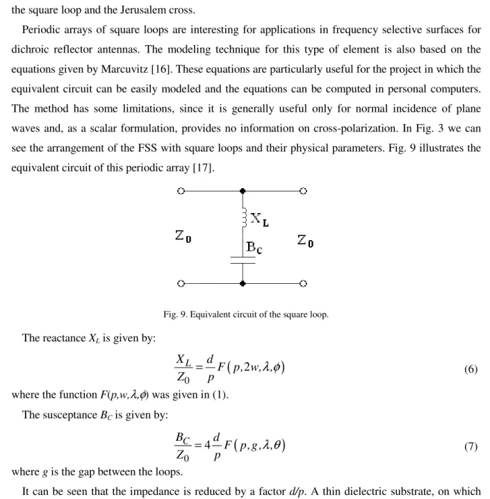
waves and, as a scalar formulation, provides no information on cross-polarization. In Fig. 3 we can
see the arrangement of the FSS with square loops and their physical parameters. Fig. 9 illustrates the
equivalent circuit of this periodic array [17].
Fig. 9. Equivalent circuit of the square loop.
The reactance XL is given by:
(
)
0
2 L
X d
F p, w, ,
Z = p
λ φ
(6)where the function F(p,w,λ,φ) was given in (1).
The susceptance BC is given by:
(
)
0
4 C
B d
F p,g , ,
Z = p
λ θ
(7)where g is the gap between the loops.
It can be seen that the impedance is reduced by a factor d/p. A thin dielectric substrate, on which
the conductive elements are printed, causes an increase in the susceptance of the array while no effect
on the inductive reactance is observed. Equation (7) is corrected to:
(
)
0
4
C r
B
d
F p,g , ,
Z
=
ε
p
λ θ
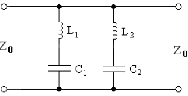
(8)The equivalent circuit model for the Jerusalem cross, consisting of a combination of two LC
Fig. 10. Equivalent circuit of the Jerusalem cross.
The value of each inductive strip with width w, counting from L1, is calculated using a conventional
equation given by Marcuvitz. The susceptance B1 is calculated as the sum of two susceptances Bg and
Bd. Bg is the susceptance due to the capacitance between the capacitors final horizontal spaced of g,
reduced by a factor of d/p. This susceptance is calculated as:
((((
))))
4, ,
g
d
B F p g
p
λ
= = =
= (9)
The susceptance Bd is given by the final capacitor spaced by
((((
p−−−−d))))
and it is calculated as:((((
))))
((((
))))
4 2
,
,
dh
g
B
F p p
d
p
λ
+
+
+
+
=
−
=
−
=
−
=
−
(10)The value of C2 is not calculated directly using the analysis as described above, but from the
assumption of a dipole resonance frequency f3, such that, where is the resonant wavelength. From the
value, C2 is derived from the equation of the resonant circuit in series as:
3 2 2
1
2
f
L C
π
=
=
=
=
(11)The inductive reactance XL2 is due to strips of length d is calculated as:
(
)
2 0 2 L X dF p, w, ,
Z = p
λ θ
(12)V. RESULTS
To illustrate how the software works, we will make comparisons with the simulated results obtained
by the software and measured results found in some references.
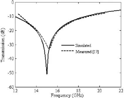
Fig. 11 illustrates a comparison between the results obtained with the software with the measured
results presented in [17] for transmitted in dB. The dimensions of the structure were: w = 0.47 mm, g
= 0.25 mm, d = 5mm, p = 5.25 mm, and εr = 1.24. The element was the square loop. Considering the
resonance frequency, for measured results it occurs at 15.25 GHz while for simulated results it occurs
at 15 GHz (error = 1.64%). Considering the bandwidth at – 20 dB, for measured results it was 2.03
GHz while for simulated results it was 2.06 GHz (error = – 1.48%). So, the results obtained by the
Fig. 11. Comparison between simulated and measured results of a square loop FSS.
Fig. 12 illustrates a comparison between the results obtained with the software with the measured
results presented in [18] for transmission in dB. The dimensions of the structure were: w1 = 0.15 mm,
w2 = 0.15 mm, g = 0.60 mm, d = 3.70 mm, p = 5.05 mm, and εr = 1.24. The element was the gridded
square loop. Considering the resonance frequency, for measured results it occurs at 23.08 GHz while
for simulated results it occurs at 23.18 GHz (error = 0.43%). Considering the bandwidth at – 20 dB,
for measured results it was 1.49 GHz while for simulated results it was 1.31 GHz (error = 12.1%).
Again, the results obtained by the software agree with the measured for prediction of resonance
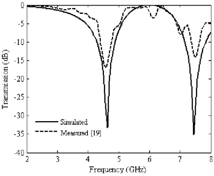
resonance occurs at 7.44 GHz. For the measured results [19], the first resonance occurs at 4.58 GHz
and the second resonance occurs at 7.52 GHz. For the first resonance the error was – 1.09% and for
the second resonance the error was 1.06%. The levels in the resonance frequencies differ by about 20
dB. This may be due to an inadequate process of measuring or because the equivalent circuit is an
approximate method, or a combination of both, but a good prediction of the resonance frequencies and
curve shape was achieved.
Typical frequency characteristics for transmission through a Jerusalem cross grid at normal
incidence are shown in Fig. 14. The dimensions of the structure were: w = 0.90 mm, d = 4.95 mm, p =
6.50 mm, g = 0.21 mm, h = 0.30 mm and εr = 1.24. The main features of the response are the rejection
frequency bands corresponding to resonances at f1 and f3. For measured results [15], the first
resonance occurs at 11.62 GHz and the second resonance occurs at 33.82 GHz. For simulated results,
the first resonance occurs at 11.10 GHz and the second resonance occurs at 33.00 GHz. Considering
the resonance frequency, for the first resonance the error was 4.48% and for the second resonance the
error was 2.42%. As we can see, both numerical methods presented a good agreement.
Fig. 14. Comparison between simulated and measured results of a Jerusalem cross FSS.
VI. EXPECTED RESULTS WITH THE SOFTWARE
The authors intend to use the software in the special topics course, frequency selective surfaces,
given in the Post-graduate Program in Electrical Engineering and Computing, at Federal University of
Rio Grande do Norte. The idea is to provide the software on the course webpage and apply lists of
exercises that can be solved using the software. The lists will be directed to students so that they can
understand how the physical parameters and the geometry of the structures influence the transmission
characteristics of a FSS. This could be done with commercial softwares such as Ansoft DesignerTM or
CST Microwave StudioTM, for example, which uses full-wave methods to perform the analysis of the
structures, but the high cost of the license becomes our software very attractive. In addition, the low
computational effort required by the equivalent circuit method allows a faster resolution of the lists of
exercises. At the end of the semester, questionnaires will be used to diagnose the effectiveness of
educational software use in the FSS.
VII. CONCLUSIONS
This work has described frequency selective surface simulation software, using equivalent circuit
model, designed for student training. The authors hope that the software will improve students’
knowledge of the relationships between FSS parameters. The tool provides students the opportunity to
investigate FSS with different elements shapes, modifying its design parameters and obtaining the
results for each of these modifications. The authors intend to use the software in a special topics
Education, vol. 49 (3), pp. 404-414, Aug. 2006.
[5] D. Gurkan, A. Mickelson and D. Benhaddou, “Remote Laboratories for Optical Circuits”, IEEE Trans. On Education, vol. 51 (1), pp. 53-60, Feb. 2008.
[6] J. F. Haffner, L. F. A. Pereira and D. F. Coutinho, “Computer-Assisted Evaluation of Undergraduate Courses in Frequency-Domain Techniques for System Control”, IEEE Trans. On Education, vol. 49 (2), pp. 224-235, May 2006.
[7] J. F. Guerrero, M. Bataller, E. Soria and R. Magdalena, “BioLab: An Educational Tool for Signal Processing Training in Biomedical Engineering”, IEEE Trans. On Education, vol. 50 (1), pp. 34-40, Feb. 2007.
[8] M. Duarte, B. P. Butz, S. M. Miller and A Mahalingam, “An Intelligent Universal Virtual Laboratory (UVL)”, IEEE Trans. On Education, vol. 51 (1), pp. 2–9, Feb. 2008.
[9] B. Ramamurthy, “GridFoRCE: A Comprehensive Resource Kit for Teaching Grid Computing”, IEEE Trans. On Education, vol. 51 (1), pp. 10-16, Feb. 2007.
[10]T. K. Wu, Frequency Selective Surface and Grid Array, New York, NY: John Wiley & Sons, 1995.
[11]J.P. Gianvittorio, J. Romeu, S. Blanch, and Y. Rahmat-Samii, “Self-similar prefractal frequency selective surfaces for multiband and dual-polarized applications”, IEEE Trans. Antennas Propag., vol. 51, pp. 3088-3096, 2003.
[12]J. Romeu and Y. Rahmat-Samii, “Fractal FSS: A novel dual-band frequency selective surface”, IEEE Trans. Antennas Propag., vol. 48, pp.1097-1105, 2000.
[13]J. Romeu and Y. Rahmat-Samii, “Dual band FSS with fractal elements”, Electron. Lett., vol. 35, pp. 702-703, 1999.
[14]I. Anderson, “On the theory of self-resonant grids”, Bell Syst. Tech., vol. 54 (10), pp. 1725-1731, 1975.
[15]R. J. Lagley and A. J. Drinkwater, “An Improved empirical model for the Jerusalem cross”, IEE Proc., Part H: Microwaves, Opt. Antennas, vol. 129 (1), pp. 1-6, 1982.
[16]N. Marcuvitz, Waveguide Handbook, Editor McGraw-Hill, New York, 1951.
[17]R. J. Langley and E. A. Parker, “Equivalent circuit model for arrays of square loops”, Electronics Letters, vol. 18 (7), 294-296 (1982).
[18]C. K. Lee e R. J. Langley, “equivalent-Circuit Models for Frequency-Selectvie Surfaces at Oblique Angles of Incidence”, IEE Proceedings, vol. 132 (6), 395 - 399 (1985).