Abstract— An improved microwave method to extract the complex
permittivity of solid and liquid materials filled in a short-circuited waveguide is developed. The method determines accurately the dielectric constant of thin and moderate thick samples. It eliminates the problems arising from any position offset of the dielectric slab in transmission / reflection methods. The proposed method is iterative and the initial value is calculated by using the 7th approximation order of trigonometric terms in the exact reflection coefficient equation. This approach is applied to the simulated data of low loss and dissipative materials in limited frequency band.
Index Terms—Complex permittivity, Rectangular waveguide, Thin materials,
X band.
I. INTRODUCTION
In the microwave frequencies, the electrical and magnetic properties of the dielectric medium are
strongly influenced by the frequency. Given that the increased use of nanocomposite materials, there
is a growing industrial demand for dielectric characterization of these new materials, starting from the
designing phase through the control process via the production stage. Therefore, the knowledge of the
constituent concentrations (resin binder, carbon black filled epoxy polymer),
provides
the ability tosize the desired dielectric properties of the composite materials. However, there is a growing demand
for accurate microwave techniques to characterize solids, liquids and granular materials over
broadband frequencies and at different temperatures [1], [2], [3], [4].
Various microwave methods are proposed in literature with their advantages and drawbacks.
Although the resonant techniques [5], [6], [7]are more accurate than the nonresonant techniques [8],
[9], they require a meticulous sample preparation of the material under test. Practically, this is no
longer
appreciated
. The nonresonant methods are widely used to characterize different kinds ofmaterials over a broad frequency band. However, they require a less sample preparation compared to
resonant methods. Due to its simplicity, the nonresonant waveguide transmission / reflection method
is presently the most widely used broadband measurement technique; it is also applied for measuring
the dielectric constant of thin materials [10], [11], [12], [13].
In this regard and in accordance with the transmission and/or reflection techniques, K. Sarabandi
A
Microwave Method for Complex
Permittivity Extraction of Thin Materials
Nawfal Jebbor
Spectrometry Laboratory of Materials and Archeomaterials (LASMAR) Faculty of Sciences, Moulay Ismail University, Meknes – Morocco
[email protected] Seddik Bri
Electrical Engineering Department, Technology High School (ESTM), Moulay Ismail University, Meknes- Morocco
and his co-worker F. T. Ulaby have based, in their paper [12], on measuring the reflection coefficient
Γ of a thin sample filled in a rectangular waveguide. The exact expression of Γ is simplified in the case of thin materials and they obtain an explicit expression of the first and second orders of the
relative dielectric constant εr. But a small offset positioning of the slab inside the waveguide will
generate enormous errors in the inversion of εr from the measured Γ. On the other hand, in the article
of B. K. Chung [13], the relative permittivity determination is performed from the measured
transmission coefficient T. Chung obtains an explicit expression of εr via a second order
approximation. Moreover, his method eliminates to a certain level of achievement the offset
positioning problem encountered in Sarabandi technique. In this article, we present a method to
characterize thin dielectric materials by measuring the reflection coefficient of a short-circuited
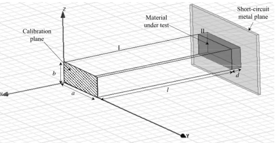
rectangular waveguide shown in Fig. 1.
l
d b
a
I
II Calibration
plane
Material under test
Short-circuit metal plane
Fig. 1. Illustration of the problem. Rectangular waveguide with a dielectric slab material occupying region II (between x=-l and x=-(l+d)).
The slab under test is in direct contact with the metal plane of short-circuit without air gap and the
offset positioning problem is definitively eliminated. The trigonometric terms of the exact expression
of Γ are linearized in the case of thin materials and one complex relative permittivity value is
extracted. This technique uses higher order approximations and the accuracies are compared to the
true value of dielectric slab and to Sarabandi / Chung approximations. In one objective to get a
relative permittivity as accurately as possible, the exact expression of Γ is solved by
Newton-Raphson method with an initial guess of the iterative process is εr which is a solution of the
approximated equation of Γ. However, the initial value problem encountered in iterative techniques is
thus overcome. Once the initial guess is known, one can proceed to another traditional measurement
[14] for the case where it is possible to fill the entire sample holder with the material under test (liquid
or solid). By using the electromagnetic 3D-simulation software Ansoft HFSS, the studied structure of
Fig. 1 is implemented and the relative dielectric constant of Teflon, wood and distilled water are
extracted via the proposed method. The experimental setup can help immensely to characterize new
nanocomposite materials mainly in microwave frequencies and in a wide range of temperatures [1],
II. COMPLEX PERMITTIVITY THEORY DEVELOPMENT
Consider a short-circuited rectangular waveguide of dimensions (a×b) containing a thin slab placed
in a plane orthogonal to the propagation direction Ox and in direct contact with the short-circuit plane
as shown in Fig. 1. In the analysis, the sample is assumed isotropic, symmetric, homogeneous and
non-magnetic (µr=1). The dielectric slab of thickness d is located at x=-l. l is the distance between the
calibration plane and the air-sample interface. In an objective to seek a relationship between the
reflection coefficient S11=Γand the relative permittivity εr=εr’-jεr” of the dielectric slab material, we
shall develop expressions of electric and magnetic fields in regions I and II from their potentials A
and F such as [10], [11], [15]:
) F . ( 1 j F j A 1 H F 1 ) A . ( 1 j A j E r 0 0 0 r 0 r 0 0 ∇ ∇ ε ε ωμ − ω − × ∇ μ = × ∇ ε ε − ∇ ∇ ε ε ωμ − ω − = (1) (2)
Where
ε
0andμ
0are the permittivity and permeability of free-space respectively. Assuming thatthe rectangular waveguide operates in the dominant mode TE10, we have A = 0and ∂Fx/∂y=0
[15]. Then, the electric vector potential can be written for regions I and II as:
[
]
[
C e x C e x]
-l-d x l ) a z cos( ) z , x ( F 0 x l x e C x e C ) a z cos( ) z , x ( F 4 3 ) II ( x 0 2 0 1 ) I ( x − ≤ ≤ γ − + γ π = ≤ ≤ − γ − + γ π = (3) (4)Where γ0 = j2π/λ0 1−λ20/λ2c, γ= j2π/λ0 εr −λ20/λ2c (5)
λ0= c/f and λc= c/fc correspond to the free space and cut-off wavelengths; and f, fc and c are the operating and cut-off frequencies and the speed of light in vacuum, respectively. The time factor
t j
eω was assumed and suppressed. The unknown coefficients C1, C2, C3 and C4 can be obtained by
applying the appropriate boundary conditions at x=-l and x=-(l+d). C1 and C2 represent the
magnitudes of the incident and reflected waves in region I; C3 and C4 represent the magnitudes of the
incident and the reflected waves in region II.
The complex reflection coefficient S11 is found to be:
0 0 2 1 2 11 / ) d tanh( / ) d tanh( R C C S γ γ + γ γ γ − γ = = Γ = (6)
Where
R
=
e
−γ0lis the transformation factor from the air-sample interface to calibration plane. For
thin materials case, (γd) is small, and the hyperbolic tangent terms of (6) can be approximated by:
7 5 3 ) d ( 315 17 ) d ( 15 2 ) d ( 3 1 ) d ( ) d
Multiple constant propagation values γi can satisfy the approximated expression of (6); noted (6-7).
High accurate results can be attained by increasing the degree of the approximation in (6-7), and by
using “solve” function of MATLAB, we can find γi solutions of (6-7). The choice of the unique εr will
build on the solution γ=α+jβ of (6-7) that represents the best propagated mode (γ corresponds to the
smaller α-value of the solutionsγi with β is positive).
III. SENSITIVITY TO SAMPLE THICKNESS
In this
section
, the objective is focused on the accuracy of the approximated expression (6-7) whichdepends greatly on the magnitude of (γd). To analyze the sensitivity, we compute the exact reflection
coefficient S11 using equation (6) and apply it in (6-7) to find the approximate solution εr. The
solutions of (6-7) that correspond to the third, the fifth and the seventh approximation orders of tanh
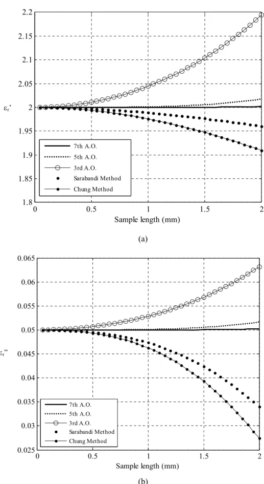
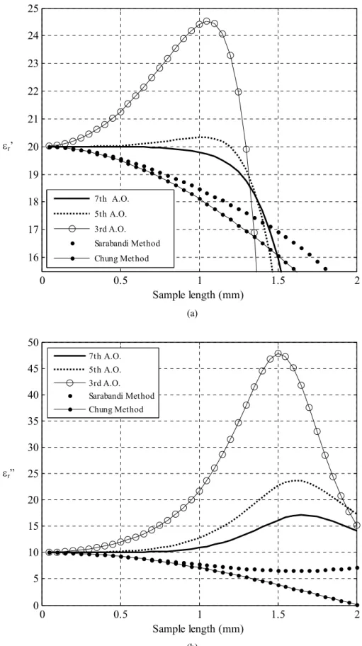
terms are compared with Sarabandi and Chung techniques for various cases. For example, Fig. 2 and
3 demonstrate the dependency of εr of a low loss sample (εr=2-j0.05) and a lossy sample (εr=20-j10)
versus the dielectric slab lengths.
The test parameters are f=10GHz and fc=6.555GHz (a WR-90 waveguide with a=22.86 mm and
b=10.16 mm is assumed). In Fig. 2, we
observe
that the 5th approximation order (5th A.O.) providesvalues that are within 0.07% of εr’ and within 0.2% of εr” for d≤1 mm. However, the 7th
approximation order (7th A.O.) provides more accurate values of εr’ and εr” for low loss materials than
the 5th A.O. In contrast, and for lossy materials (e.g. εr=20-j10), the results reported in Fig. 3 show
that only the 7th A.O. leads to values within 1% of εr’ and within 1.6%
of
εr” for d≤1 mm. The 3rd andthe 5th A.O.; and Sarabandi/Chung techniques are inaccurate and inadequate for approximating
complex value of εr for lossy materials that the thickness is more than 0.25 mm. It is seen from Fig
.
2and 3 that while the Sarabandi reflection method [12] and the Chung transmission method [13] extract
roughly similar results for εr. Our proposed method determines much better εr values for thin slab
lengths.
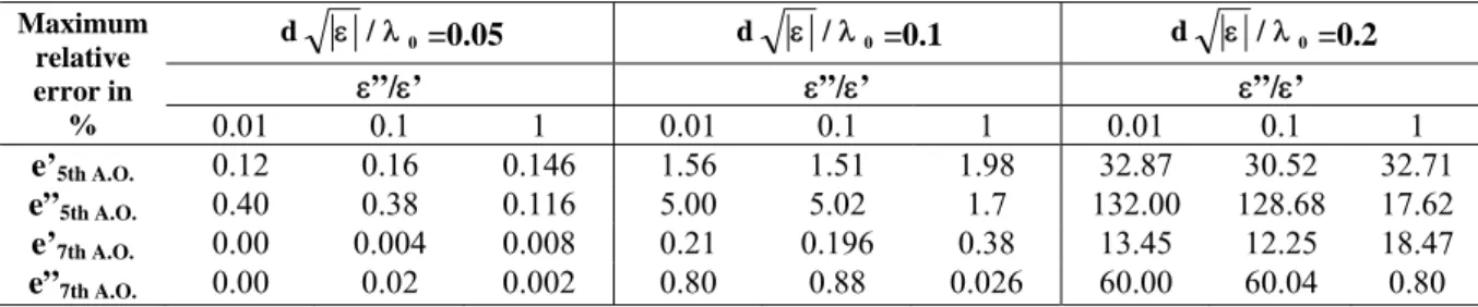
A summary of relative accuracies of the 5th and 7th A.O. are presented in Table I for slab
thicknesses d equal to 5%, 10% and 20% of λ0 / ε . The data of the table are the maximun realtive
errors defined as : e’=Max(|(εr’-ε’)/ ε’|)×100. Where εr’ and ε’ are the real parts of the εr-approximate
solution of (6-7) and the exact value of the dielectric slab respectively. All entries are computed
considering three virtual materials 5-j5, 5-j0.5 and 5-j0.05 at f=10GHz. In Fig. 4, we present the
sensitivity of the 7th A.O. of expression (6-7) to the thickness d as a function of three frequency points
8.2 GHz, 10 GHz and 12.4 GHz. However, the method is well suited for very low loss materials, and
estimating εr’ can be extended to 6 mm sample thickness at the first frequency point (f=8.2GHz). This
can be very useful when we do not know the initial value for iterative calculation techniques to
0 0.5 1 1.5 2 1.8
1.85 1.9 1.95 2 2.05 2.1 2.15 2.2
Sample length (mm) 7th A.O.
5th A.O.
3rd A.O.
Sarabandi Method
Chung Method
(a)
0 0.5 1 1.5 2
0.025 0.03 0.035 0.04 0.045 0.05 0.055 0.06 0.065
Sample length (mm)
7th A.O. 5th A.O. 3rd A.O. Sarabandi Method Chung Method
(b)
Fig. 2. Dependency of the relative permittivity ((a) real part, and (b) imaginary part) of a lowloss material (ε=2-j0.05) versus sample length. The 3rd, 5th and 7th approximation orders (A.O.) of the proposed method are comapared to
Sarabandi-reflection method [12] and Chung-transmission method [13]. εr’
0 0.5 1 1.5 2 16
17 18 19 20 21 22 23 24 25
Sample length (mm) 7th A.O.
5th A.O.
3rd A.O.
Sarabandi Method
Chung Method
(a)
0 0.5 1 1.5 2
0 5 10 15 20 25 30 35 40 45 50
Sample length (mm) 7th A.O.
5th A.O.
3rd A.O. Sarabandi Method
Chung Method
(b)
Fig. 3. Dependency of the relative permittivity ((a) real part, and (b) imaginary part) of a lossy material (ε=20-j10) versus sample length. The 3rd, 5th and 7th approximation orders (A.O.) of the proposed method are compared to Sarabandi-reflection
method [12] and Chung-transmission method [13]. εr”
Maximum relative error in
%
0
/
d ε λ =0.05 d ε /λ0=0.1 d ε /λ0=0.2
ε”/ε’ ε”/ε’ ε”/ε’
0.01 0.1 1 0.01 0.1 1 0.01 0.1 1
e’5th A.O. 0.12 0.16 0.146 1.56 1.51 1.98 32.87 30.52 32.71
e”5th A.O. 0.40 0.38 0.116 5.00 5.02 1.7 132.00 128.68 17.62
e’7th A.O. 0.00 0.004 0.008 0.21 0.196 0.38 13.45 12.25 18.47
e”7th A.O. 0.00 0.02 0.002 0.80 0.88 0.026 60.00 60.04 0.80
0 2 4 6 8 10
1 1.5 2 2.5 3 3.5 4 4.5 5 5.5 6
Sample length (mm)
8.2 GHz 10 GHz 12.4 GHz
Fig. 4. Dependency of εr’ of a lossless material (ε=2.1-j0.0016; Teflon) versus sample
length. The 7th A.O. solutions are computed for three frequency points: 8.2 GHz, 10 GHz and 12.4 GHz.
IV. HFSS SOFTWARE SIMULATIONS
HFSS is a high performance full wave electromagnetic field simulator for 3D modeling structures.
HFSS can be used to calculate scattering parameters, resonant frequency and fields. In industry, HFSS
is the tool for high productivity research and development. HFSS is based on the finite element
method which computes the electromagnetic fields in the frequency domain by solving Maxwell's
equations locally. The 3D structure of Fig. 1 is designed and electromagnetic properties have been
assigned to each object:
• Microwave source is assigned to the calibration plane.
• Perfect electrically conducting (PEC) walls are assigned to all external surfaces except source.
• Air electromagnetic properties are assigned the inner volume of region I.
• Electromagnetic properties of the material under test are assigned to the inner volume of region II.
The HFSS simulations are performed for 40 frequency points from 8.2GHz to 12.4GHz. Then, S11
parameter data file is exported and incorporated into MATLAB program in order to recover the
software material properties of the material under test via the proposed method.
V. NUMERICAL VALIDATION
The waveguide structure of the Fig. 1 has been simulated by the Ansoft HFSS software. The
reflection coefficient S11 is computed at the calibration plane for 40 X-band frequency points. The
numerical results of S11 are thereafter incorporated into MATLAB program to retrieve the starting
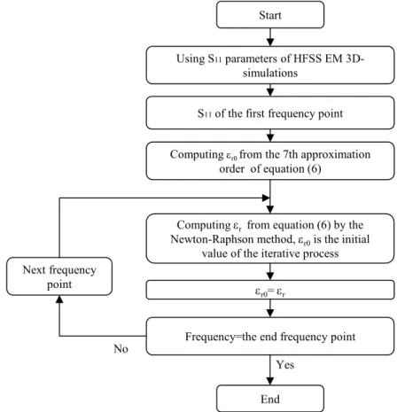
relative permittivity. The flowchart of the Fig. 5 describes the algorithm of MATLAB program.
The solving iterative process of equation (6) is started with an initial value εr0 which is a solution of
the 7th A.O. of equation (6-7). The starting S11 corresponds to the lowest frequency point. This choice
is based on the results of Fig. 4 and helps to extract the dielectric constant of materials as thick as
possible. εr0 is the initial value of the first loop and εr0 of the next loop is equal to εr that is the solution
of the previous iteration. We note that the equation (6) is resolved iteratively by the Newton-Raphson
method. We check the proposed method for Teflon, wood and distilled water. For liquid
characterization case, the experimental setup of Fig. 1 is positioned vertically. But for this paper, we
will deal only the numerical validation of the proposed approach. The flowchart of Fig. 5 summarizes
all steps in totality including the HFSS simulation results and the iterative calculation by MATLAB.
Start
Using S11parameters of HFSS EM
3D-simulations
Computingεr0from the 7th approximation
order of equation (6) S11of the first frequency point
Computingεr from equation (6) by the
Newton-Raphson method, εr0is the initial value of the iterative process
εr0= εr
Frequency=the end frequency point Next frequency
point
End Yes No
• Waveguide WR-90.
• Distance between calibration plane and air-sample interface l=70 mm. • Frequency range: [8.2–12.4] GHz (X-band).
• Sample thicknesses: d=5 mm for Teflon, d=2 mm for wood and d=1 mm for distilled water.
• The inner walls of waveguide are assumed perfectly conductor.
The numerical results of relative complex permittivity of Teflon, wood and distilled water are
presented graphically in Fig. 6, 7 and 8 respectively. The results of the distilled water are compared
with the theoretical Debye model values [3]. And the results of the wood slab are compared with the
measured data obtained by the Transmission / Reflection method [8] of 10 mm wood sample
thickness. To do these comparisons, the Debye model and measured data are incorporated in the
simulated material properties.
All findings values agree well with the published data [3], [8], [13] and measurements. Generally,
the numerical methods require an initial guess to obtain a convergence to the exact permittivity of the
material under test. But the results reported in Fig. 6, 7 and 8 are obtained by the initial values εr0. As
indicated previously, εr0 is calculated by the 7th A.O. equation. However, we do not need any
information about the εr range. It is seen from Fig. 6, 7 and 8 that we can retrieve the relative
permittivity of thin or thick simulated materials from their S11 parameter. For very low loss materials,
the uncertainty of S11 increases greatly for very thin samples. The solution might be cutting the
sample with a few millimeters thick. For the other extreme case, i.e. for very high loss materials, thick
samples might absorb all the electromagnetic wave energy. However, the certainty to determine
accurately εr is very low. The solution might be cutting the sample with a thickness less than one
millimeter.
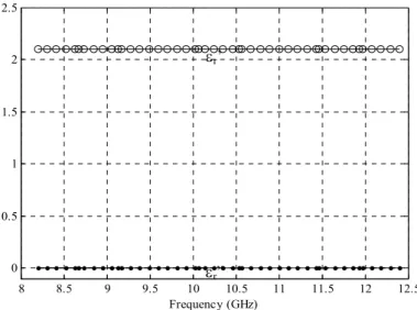
8 8.5 9 9.5 10 10.5 11 11.5 12 12.5
0 0.5 1 1.5 2 2.5
Frequency (GHz)
Fig. 6. Simulated relative complex permittivity of 5 mm long Teflon sample by the proposed method.
εr’
8.5 9 9.5 10 10.5 11 11.5 12 2.6
2.62 2.64 2.66 2.68 2.7 2.72 2.74 2.76 2.78
Frenquency (GHz)
Measured data by the T/R method [8] Simulation data
8.5 9 9.5 10 10.5 11 11.5 12 0.2
0.22 0.24 0.26 0.28 0.3 0.32 0.34 0.36 0.38 0.4
Frenquency (GHz)
Measured data by the T/R method [8] Simulation data
(a) (b)
Fig. 7. (a) and (b) are the real and imaginary parts of the relative complex permittivity of wood sample respectively. The plots represent a comparison between the simulation and the measured results of 2 mm and 10 mm wood sample thicknesses
respectively. We note that the measured data are obtained by the Transmission / Reflection (T/R) method [8] and incorporated in the simulated material properties. The simulation results are performed by the proposed method.
8 8.5 9 9.5 10 10.5 11 11.5 12 12.5 56
58 60 62 64 66 68
Frequency (GHz)
Simulation Data Debye Model
8 8.5 9 9.5 10 10.5 11 11.5 12 12.5 26
27 28 29 30 31 32 33 34
Frequency (GHz) Simulation Data
Debye Model
(a) (b)
Fig. 8. Simulated relative complex permittivity ((a) real part and (b) imaginary part) of 1 mm distilled water thickness by the proposed method. The results are compared with Debye model.
VI. CONCLUSION
An improved method is developed for complex permittivity determination of thin and moderate
thick liquid and solid materials. The samples are in direct contact to the metal plane of the
short-circuited rectangular waveguide without any air gap. The dielectric constant is then calculated from
the simulated complex reflection coefficient at the input of the waveguide section. The errors arising
from any position offset of the sample are eliminated. The method approximates the hyperbolic
tangent terms which produce multiple solutions for complex permittivity determination; and the
unique solution that corresponds to the best propagated mode is selected. High accurate solution can
be attained by increasing the degree of the approximation. Then, this εr-solution is considered as an
initial value of the iterative process resolving the exact expression of the reflection coefficient.
However, the complex permittivity is determined more accurately. The method is verified numerically
εr’ εr”
permittivity values integrated in simulations. The experimental validation will be performed in the
near future.
REFERENCES
[1] D. Michali, C. Apollo, R. Pastore, and M. Marchetti, “X-Band microwave characterization of carbon-based nanocomposite material, absorption capability comparaison and RAS design simulation,” Composites Science and Technology, vol. 70, pp. 400-409, Nov. 2010.
[2] H. Ebara, T. Inoue, and O. Hashimoto, “Measurement method of complex permittivity and permeability for a powdered material using a waveguide in microwave band,” Science and Technology of Advanced Materials, vol. 7, pp. 77-83, Feb. 2006.
[3] U. C. Hasar, O. Simsek, M. K. Zateroglu, and A. E. Ekinci, “A microwave method for unique and non-ambiguous permittivity determination of liquid materials from measured uncalibrated scattering parameters,” Progress In Electromagnetics Research PIER, vol. 95, pp. 73-85, 2009.
[4] A. Mdarhri, M. Khissi, M. E. Achour, and F. Carmona, “Temperature effect on dielectric properties of carbon black filled epoxy polymer composites,” Eur. Phys. J. Appl. Phys., vol. 41, pp. 215-220, Apr. 2008.
[5] L. F. Chen, C. K. Ong, C. P. Neo, V. V. Varadan, and V. K. Varadan, Microwave Electronics Measurement and Material Characterization, John Willey and Sons, West Sussex, England, 2004, 37.
[6] C. P. Rubinguer, and L. C. Costa, “Building a resonant cavity for the measurement of microwave dielectric permittivity of high loss materials,” Microwave Opt. Tech. Lett., vol. 49, pp. 1687-1690, July. 2007.
[7] E. Li, Z. P. Nie, G. Guo, Q. Zhang, Z. Li, and F. He, “Broadband measurements of dielectric properties of low-loss materials at high temperatures using circular cavity method,” Progress In Electromagnetics Research, PIER, vol. 92, pp. 103-120, 2009.
[8] N. Jebbor, S. Bri, L. Bejjit, A. Nakheli, M. Haddad, and A. Mamouni, “Complex permittivity determination with the transmission / reflection method,” Int. J. Emerg. Sci., vol. 1(4), pp. 682-695, Dec. 2011.
[9] U. C. Hasar, “A fast and accurate amplitude-only transmission-reflection method for complex permittivity determination of lossy materials,”IEEE Transactions on Microwave Theory and Techniques, vol. 56, pp. 2129-2135, 2008.
[10]U. C. Hasar, “Permittivity measurement of thin dielectric materials from reflection-only measurements using one-port vector network analyzers,” Progress In Electromagnetics Research, PIER, vol. 95, pp. 365-380, 2009.
[11]U. C. Hasar, and O. Sismek, “An accurate complex permittivity method for thin dielectric materials,” Progress In Electromagnetics Research, PIER, vol. 91, pp. 123-138, 2009.
[12]K. Sarabandi, and F. T. Ulaby, “Technique for measuring the dielectric constant of thin materials,” IEEE Transactions on Instrumentation and Measurement, vol. 37 pp. 631-636, Dec. 1988.
[13]B. K. Chung, “Dielectric constant measurement for thin materials at microwave frequencies,” Progress In Electromagnetics Research, PIER, vol. 75, pp. 239-252, 2007.
[14]J. Baker-Jarvis, Transmission/reflection and short-circuit line permittivity measurements, NIST Note 1341. U.S. Government Printing Office, Washington, D.C., July 1990.