Abstract
Control of time delay integrating systems is a challenging and on-going research. In this paper a new structure for control of stable and integrating time delay systems is presented. The control de-sign process is as simple as selection of some constant gains, for which simple formulae are introduced. The design methods are derived analytically, while no fractional approximation for the time delay term of the plant transfer function is used. Simulation, as well as, experimental studies reveal the exceptional effectiveness of the proposed methods in achieving a robust and well-performing tracking, even when the plant pure time delay is very large.
Keywords
Time-delay systems; Integrating processes; Tuning formulae; Un-certainty; Robustness; Input cost; Servo/regulator tradeoff.
Simple Formulae for Control of Industrial Time Delay Systems
1 INTRODUCTION
Time delay is very often encountered in various industrial systems, such as pneumatic and hydrau-lic networks, chemical processes, long transmission lines, robotics, etc. A large group of industrial processes are stable, with a possible integrating and time delay nature, e.g., in a fluid level or distil-lation column level control problems (Alfaro and Vilanova, 2012). Control of time-delay systems has always been difficult, and if the system has integrating characteristics, this difficulty would be dou-bled, for the balanced relationship between the input and output may be easily destroyed by an external disturbance (Liu and Gao, 2011).
Smith predictor is one the oldest and most popular methods of control for time delay systems. Although the original method is only applicable to stable systems (Smith,1959), more recent devel-opment on the Smith structure can be applied to unstable time delay systems as well. Some of such methods are limited to integrating first order pure time delay systems (IFOPTD) (Kaya, 2003; Majhi and Atherton, 2000; Normey-Rico and Camacho, 2009; Shamsuzzoha and Moonyong , 2008; Uma and Rao , 2014) and some others involve complex algorithms (Garca andAlbertos, 2008; Hang,
Moslem Azamfar a Amir H. D. Markazi b,*
a,b Digital Control Laboratory., School of
Mechanical Engineering, Iran University of Science and Technology, Tehran, Iran. a [email protected]
Corresponding author: * [email protected]
http://dx.doi.org/10.1590/1679-78253032
Wang and Yang, 2003; Kwak, Sung and Lee, 2001; Matausek andMicic, 1996; Matausek andRibi, 2012). Due to such complexities, compared to the original Smith Predictor, discrete-time version of time-delayed plants are used in many practical applications (Garca andAlbertos, 2013; Normey-Rico and Camacho, 2009; Torrico andNormey-Rico, 2005).
Application of PID controllers for time delay systems are proposed by many other researchers, although they are either applicable to stable plants such as in (Cvejn, 2013) or do not provide ac-ceptable tracking and disturbance rejection properties (Ali andMajhi, 2010; Shamsuzzoha andLee, 2007; Wang, Hang and Yang, 2001). Since most of the PID-based methods, are based on the Pade' approximation of the time delay term, they provide poor performance when long time delays are involved (Tan, Marquez and Chen, 2003; Vanavil, Chaitanya and Seshagiri Rao, 2015). Similarly, many methods which are based on the internal model principle, are also based on the Pade' approx-imation and, therefore, provide acceptable disturbance rejection and reference tracking properties only for rather small time delays (Jin and Liu, 2014; Liu and Gao, 2011; Tan et al., 2003; Vanavil et al., 2015; Zhang, Rieber and Gu, 2008). Considering the well-known drawbacks of the existing methods, the objective of this paper is to provide a simple control structure with straightforward tuning guidelines, in which the closed loop performance and stability are guaranteed. The process of tuning the control parameters are very simple and only include substitution in some pre-specified formulas. The proposed method is tailored for application to the case of frequently seen industrial plants, as described in Section 2. The results of simulations are compared with some of other exist-ing methods.
This paper is organized as follows: Problem statement and the proposed control structure are given in Section 2. In Section 3, the tuning rules are given for prescribed standard plant models. Closed loop performance of the proposed method is studied in Section 4. In Section 5, the results of simulations are compared with some methods reported in the recent literatures, and their strengths and weaknesses are investigated. An experimental case study is described in Section 6 where the speed control of an AC servo motor with deliberately induced long time delay is considered. A com-parison between simulation and experimental studies is also given in Section 6. Concluding remarks are given in Section 7.
2 PROBLEM STATEMENT
Many industrial time delay stable and integrating systems can be approximated by one of the fol-lowing simplified forms (Skogestad, 2003;Shamsuzzohaa and Skogestad, 2010):
1.Pure Time Delay System (PTD):
(1)
2.First Order Pure Time Delay System (FOPTD):
(2)
(3)
4.Integrating First Order Pure Time Delay System (IFOPTD):
(4)
5.Double Integrating Pure Time Delay System (DIPTD):
(5)
where kis the system gain, τ is the time constant andis the dead time parameter.
The main purpose of this article is to provide a series of analytical tuning rules for such sys-tems, which can guarantee the closed-loop stability and an acceptable level of performance and ro-bustness.
3 PROPOSED METHOD
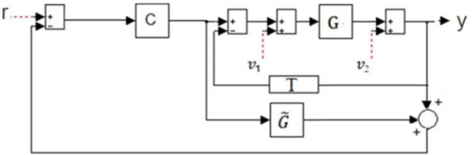
The proposed control structure is shown in Figure 1. In this figure,
R
is the reference input,v
1is the plant input disturbance,v2is the plant output disturbance,y
is the system output,T(s)is the innerloop stabilizing controller,C(s)is the main forward controller, andG~(s)is a feed-forward controller.
The closed-loop response of the system in Figure 1, is given by
( ) 2~ ) ( 1 1 ) ( ~ ) ( 1 ) ( ) ( ) (
= v
s s G s C v
s s G s C s G r s
s G s C y
(6)
where,
s =1C(s)G(s)C(s)G~(s)T
s
1C(s)G~(s)
G(s) (7)
The inner loop controllerT(s)is designed to guarantee the internal stability. Simple formulae for
the controllersC(s)andG~(s)are introduced, such that the closed-loop stability and performance of the systems 1-5 are guaranteed.
For each of the systems (1)-(5), suitable controllers and tuning rules are proposed in the sequel.
3.1 PTD and FOPTD Plants
Since a PTD and FOPTD plants are stable, the inner loop controller in Figure 1 can be selected as 0.
= ) (s
T Since PTD plants are special cases of FOPTD plants, with=1, similar control design
methodologies can be used for the remaining controllers, and , i.e.,
1) ( 1 1 1 = s ss s k s C d
(8) and
sp e s ks k s G
1 = ~
(9)
The closed-loop characteristic equation is then given by
p sd e s s s k s k k s
1) ( 1 1 1 1 = (10)Here, is a to-be-tuned parameter, which must be selected according to the desired trade-off between the performance, robust stability and input cost. By selecting <1, the following approx-imation holds (Skogestad, 2003)
) (
1) 1/(
s e sThen, (10) can be approximately written as
se s s s p k k d k
s ( )
1) (
1
1
(11)
By using the results in (Matausek and Micic, 1996) the following lemma can be deduced:
Lemma 1: Consider the closed loop characteristic (11). Let
1 < 0 ), ( = p k
Then, for
=kp/10, the closed loop stability is guarantied if the controller gaink
dis chosen as2 2 2 ) 2 ( ) (1 ) ( 2 = m m d k k (12)
It can be verified that, the closed-loop stability and robustness can be satisfied by selecting
typ-ical values =0.4 and m=64(Matausek and Micic, 1996), the resulting control gain would then be as
) ( 0.724 =
k
kd (13)
It also turns out that
1 = ) (
) ( ) ( lim = ) ( lim
0 s
s G s C t
y s r
t
and
0 = ) ( lim = ) (
lim y1 t yv2 t t
v
t
This provides step disturbance rejection and step tracking properties.
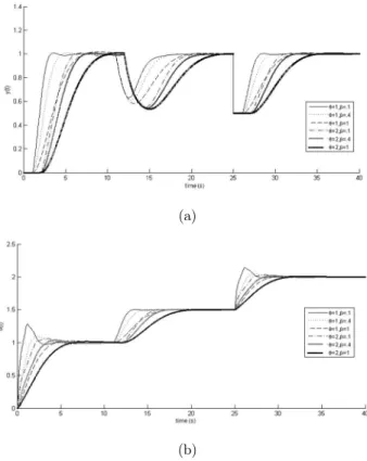
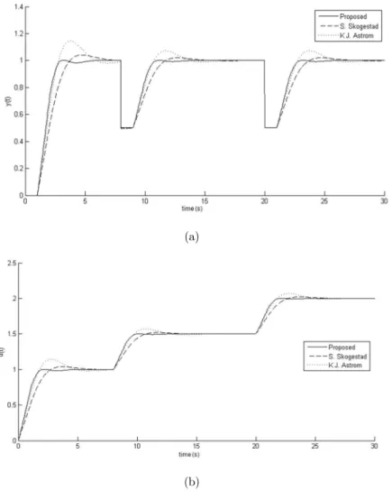
Figures 2(a) and 2(b), respectively, depict the closed-loop step response and control input for different values of
and , and for
=
1
andk=1. The time response due to two consecutive stepdisturbances at times 10sec and 25sec are also shown. It can be seen that the closed-loop settling time is increased for larger values of
. The associated resulting control input signals are also shown in Figure 2(b).(a)
(b)
3.2 IPTD Plants
In order to preserve the stability of the inner loop, a constant gain controller T(s)=ki is selected, i.e., s i e s k k s G s
T
( ) ( )=1
1 (14)
In order to achieve a phase margin of 60 and a gain margin of 3, the following gain is chosen:
k
ki=0.5236 (15)
The controllers C(s) and
G
~
(
s
)
are then obtained as
1 0.5236 1 1 1 = s e s s k s C sd
(16) and
s s p e s e k k s G
0.5236 1 = ~ (17)The resulting closed-loop denominator is
p s s
d e s e s s s k s k k
s
0.5236 1 1) ( 1 1 1 1 = (18)Again, the value of parameter kd is determined using (12). In particular, for =0.4and
4 6 =
m
,
k
d can be obtained from (13). It can be simply verified that, limtyr
t =1and
t =0 ylimt v , as is desired.
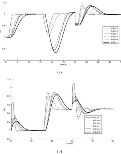
In Figure 3(a), for several values of the parameters and
,andwithk=1, the closed-loop step(a)
(b)
Figure 3: Effects ofon the time response (a) and control input (b) for k=1.
3.3 IFOPTD Plants
To preserve the stability of the inner-loop,
1 1 =
)
(
s s k s
T i
is selected, then
1
1
=
)
(
)
(
1
s
s
e
k
k
s
G
s
T
s
i
(19)
By selecting
=
/10, the effect of the low-pass filter in the above equation can be neglected for computation of the phase and gain margins; therefore, parameter ki can be obtained from (15).As before, the controllers C(s) and
G
~
(
s
)
are selected such that the closed-loop stability and performance are satisfied, i.e.,
s
d e
s s s
s s k s
C
( 1)0.5236 1
1 1 . 1 1
1) ( 1) ( 0.5236 1 = ~ s e s s e k k s G s s p
(21)The closed-loop denominator is obtained as
p s s
d e s s e s s s k s k k
s
( 1)0.5236 1 1) ( 1 1 1 1 = (22)
By using (12), the value of the parameter
k
d can be obtained. Through simulation studies,itcan be further concluded that an increase in
leads to a smoother control signal and a slower time response.3.4 DIPTD Plants
To preserve the stability of the inner-loop, 2
1) / ( 1 = ) ( s Ns T s T k s T d d i
is selected. Then,
s d d i e s Ns T s T k k s G s
T
2 1) / ( 1 1 = ) ( ) ( 1 (23)
N is a largenumber and chosensuchthat / ≪ . Also selecting =8makesthispossible to use the PD structure proposed in (Skogestad, 2003). Therefore, the control parameters are found as
a =81 0.0625
= 2 d
i nd T
k
k (24)
For retaining the closed-loop stability, disturbances rejection and reference tracking properties, the controllers C(s) and
G
~
(
s
)
can be simply obtained as(25) and
s d d s p e s Ns T s T e s k k s G 2 ( / 1) 2 1 0.0625 1 = ~ (26)
Again, the value of parameter
k
d is determined using (12). In particular, for =0.4and 4 6 =
m
,
k
d is obtained. It can be simply verified that, limtyr
t =1and limtyv
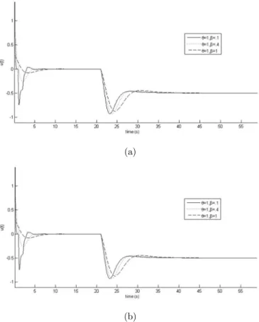
t =0, as isIn Figure 4, for several values of the parameters, =1 and withk=1, the closed-loop step re-sponse due to two consecutive step disturbances are depicted. It can be seen that, the closed-loop settling time increases for larger values of. The effects on the control signal are shown in Figure 5(a) and Figure 5(b). It can be seen that, the closed-loop performance for input tracking and dis-turbance rejection is worsened with an increase in, although it leads to a smoother control signal and reduced overshoot.
Figure 4: Effects of on the time responses, withk=1.
(a)
(b)
3.5 Performance and Robustness
Time domain performance and robustness of the proposed method are studied in this section.
3.5.1 Time Response Index
The integral absolute error (IAE), defined for the error signalyys, is an important index for as-sessment of the closed-loop system performance, which is defined as
| | (27)
Numerical solutions (by using the Matlab regression toolbox) are employed for calculation of this index for the controlled system, considering various kind of plants as described in (1)-(5). The reference and disturbance inputs are considered as unit steps. Parametric study on the effects of is also carried out and using the regression method, simple correlations with respect to are re-ported in table 1. It can be seen that, the IAE varies from 1.8 for systems given by (1)-(4), and up to of 2.8 for the system given by (5) whereas based on the results obtained from the so-called SIMC method (Skogestad, (2003)), the IAE varies from 2.17 to 7.92. The IAE(y) value for load disturbance
v
1, varies from 1.8k to3.8k
. Based on results obtained from SIMC method, the IAE value due to the disturbancev
1 varies from 2.17 to 128
3, which indicates the high sensitivity of the IAE value to an increase in the system time delay.3.5.2 Control Input
In order to evaluate the smoothness of the required control input, the index TV is defined as
1 0
= 0
= )
(
i ii
u u dt dt du u
TV (28)
This index characterizes the overall variations ofu(t), which should be reasonably small. This ensures that the un-modeled higher order dynamics of the plant is not excited by the control input.
The index TV values due to a unit step command R, and a unit step disturbance
v
1, are listed in the table 1. Based on the results, TV (u) value ranges from 1 (for PTD plants) up to 2.9 (for IFOPTD plants). Parametric study on the effects of
is also carried out and using the regression method, simple correlations with respect to
are reported in table 1.The TV(u) value for a unit step command ranges from 1 (for PTD plants), to2 2
0.1) (
21 32 .81
k
(for DIPTD plants). In deriving these
results,
=0.1was assumed. By making changes to, a desired trade-off between the time re-sponse and the smoothness of the control input can be achieved.desirable from practical point of view. Next, the control signal changes are studied through some examples and compared with required control usage of other methods.
We would see through simulation studies that some of the methods reported in the recent liter-atures require an unbounded control signal for rejection of plant output disturbances (Jin and Liu, 2014), (Alcantara et al., 2013).
3.5.3 Robustness
Sensitivity and complementary sensitivity functions, respectively denoted byS(s)andCS(s), are two conventional criteria for evaluation of closed-loop system robustness. For the general structure of the proposed controller of Figure 1, those functions are obtained as
) ( 1 = ) ( , ) (
) ( ~ ) ( 1 = )
( CS s S s
s s G s C s
S
(29)
The maximum sensitivity function is defined asMS = S(j
), the MS value is equal to theinverse of the shortest distance from point -1 in the open loop Nyquist diagram. Typical values of
S
M should be in the range of 1.4-2 (Astrom and Hagglund, 1995). Furthermore, MCS = CS(j) is inversely related to the step response overshoot, and also to the PM and GM through the follow-ing relations:
) 2 1 ( 2 ,
1
1 1
CS
CS M
sin PM M
GM
According to table 1, for each of the systems (1)-(5), MCS = 1.05, i.e., PM > 56.8 and GM >
1.95. The values of MS for DIPTD, IPTD, IFOPTD systems exceed the upper bound value of 2, yet, lead to large reductions on the IAE(y). Next, the effect of this parameter on the rejection of the input disturbance and robustness against uncertainty will be shown through some examples and compared with other methods. The controllers are designed for a nominal value of , but the actu-al vactu-alue of this parameter may change during the system’s operation. Thus, a robust controller should be effective in a wide range of uncertainty in , therefore, the term
/
can be considered as alimiton system stability. As shown in Table 1, the value of this term is 0.5 for DIPTD models, and could vary up to 1.85 for IPTD and IFOPTD models. In other words, the proposed method is robust against the time delay uncertainty of about 50% to 185%.The results obtained throughout this section are summarized in Table 1.4 SIMULATION STUDIES
Plant kd
k
i Td MSM
CS / IAEsa TVsb IAElc TVldFOPTDe ( )
0.724
k 0.04 - - - 1.756 1.05 1.85 1.8 k
6.5 1.8 k.
1
PTD (0.724)
k 0.04
- - 1.76 1.05 1.85 1.8 k1
1.9 k. 1
IPTD ) ( 0.724
k 0.04 .
0.5236
k - - 2.7 1.05 0.56 1.8
.1) (
1.52
k 3 k. 2.9
IFOPTD f k(0.724) 0.04 .
0.5236
k
/10 - 2.71 1.05 0.53 1.8 20.1) (
.4
k 2.9 k. 2.9
DIPTD (0.724 )
k 0.04 .
0.5236
k - 8. 2.73 1.05 0.5 2.8 2
2 .1) ( 21 32 0.81
k 3.8 k. 2.8
a
The IAE values for unit step command with =0.1
b
The TV values for unit step command with =0.1
c
The IAE values for unit step load disturbance,
v
1 with =0.1d
The TV values for unit step load disturbance,
v
1 with =0.1f e,
Here, for calculation ofMS,MCS,, IAElb, the assumption =4 was made. The proposed values for kd, and
i
k were obtained independent of the parameters and .
Table 1: Proposed method: Settings and performance indices for various time delay plants.
Example 1 (FOPTD plant with large dead time) Consider
e ss s G 9 1 1.5 0.5 =
which is in the form of (2). The proposed controllers are in the form of (8) and (9), for which the required parameters are very simple to find from Table 1. In particular, for=0.1, the values of
0.159 =
d
k and =0.364 are obtained.
For the purpose of comparison, the methods of Maghi (Majhi and Atherton, 2000) and Cvejn (Cvejn, 2013) are also considered, where the former approach provides controllers
s s s G s s
Gm c
1.5 1 1.5 2 = ) ( , 2 3 1 = ) (
and the latter method gives rise to the PID controller
s s s
s
C 4.5 4.5 1
6 1 = )
( 2
ance rejection. Figure 6(b) shows the control input signal for the three studied methods, based on which, the Cvejn’smethod needs a larger control input for rejection of the output step disturbance. Maghi’s method needs a non-zero control signal at the beginning, which may not be desirable from practical point of view. The required control input with the proposed control system is completely smooth and without overshoot, and for step disturbances,
v
1andv
2(see figure 6(c)) remains in an acceptable range. In order to study the robustness of the proposed method, the system responses to a unit set-point and step disturbance are illustrated in Figure 6(d), with 30% increase in the pre-sumed time delay. Results show that Maghi’s method is not resistant to time delay uncertainty and leads to instability in the closed-loop system. Cvejn’s method is more resistant to the variations of , albeit with a more sluggish time response.(a)
(c)
(d)
Figure 6: Effects of on time response (a) and control input (b) on rejection of disturbances
v
1 andv
2(c), in Example 1. Also, the time response to a unit set-point and step disturbances with +30% increase in is shown (d), which clearly shows the effectiveness of the proposed method.
Example 2 (PTD plant) Consider
= s.e s
G
which is in the form of (1). The proposed controllers are in the form of (8) and (9), for which the required parameters are found from Table 1. In particular, for
=0.1and =0.01, the values of0.685 = d
k and =0.044 are obtained.
s .5 0 = ) ( C s
and
. s .4724 0 0.16 = ) (
C s
The responses to unit step command and disturbances are shown in Figure 7(a). The achieved results show that the proposed method is superior in terms of performance indices for reference tracking and disturbances rejection. Figure 7(b) shows the control input signal for the three studied methods, where, the required control input with the proposed control system turns out to be desir-able from practical point of view.
(a)
(b)
Figure 7: Time responses due to a unit set-point and step disturbances,
v
1 andv
2(a), and the corresponding control inputs (b), in Example 2.Consider
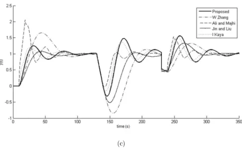
. 5 = 7.4 s e s G s which is in the form of (3). The proposed controllers are in the form of (16) and (17), for which the required parameters are found from Table 1. In particular, for =0.5, the values ofkd =0.458 ,
0.354 =
i
k and =0.316 are obtained.
The proposed method is compared with the methods of Zhang (Zhang et al., 1999), Ali (Ali and Majhi,2010), Kaya (Kaya, 2003) and Jin (Jin and Liu,2014). The method of Zhang provides the PID controller 490) (999 s 10 07 4 .365 0 = ) ( s s s C
The method of Ali gives rise to the controller
) 1 .3626 0 .626 3 3.46 2 1 .696(1 0 = ) ( s s s s C
The Kaya’s controllers, with the notation used in (Kaya,2003), are derived as
s Gc .5 0 1 1 = 1 4.43 = 2 c G and ) 4.68 0.642(1 = s
Gd
for =0.633and
m =65Finally, the PI controller obtained by the method of Jin is s s C 5.79 3 1 1 0.384 = = ) (
and the corresponding reference input filter turns out to be as
1 5.79 3 1 4.32 1 = ) ( s s s W
disturbance rejection. The method of Jin provides a good performance in set-point tracking, yet a poor performance in the rejection of plant-input disturbance.
The method proposed in this research provides very good performance in terms of set-point tracking and disturbance rejection. The required control input for the aforementioned controllers are shown in Figure 8(b). The required control input with the proposed method turns out to be superior compared to others. The control input signal with the proposed method can be further improved by tuning the
parameter, so that a better trade-off between the closed-loop performance and required control input can be achieved.In order to assess the robustness of various studied methods, a +25% perturbation in is con-sidered, and the corresponding time responses are shown in Figure 8(c). It can be concluded that the method of Kaya is not robust against perturbation in the values of , while, the method of Jin provides a good performance in reference tracking. On the other hand, the method of Ali provides a good performance in disturbance rejection, while the method proposed in this paper provides a su-perior performance compared to others.
(a)
(c)
Figure 8: Time response (a) and control input (b) for rejection of disturbances
v
1andv
2, in Example 3. Also, the time response to a unit set-point and step disturbances with +25% increase in is shown (c), which clearly shows the effectiveness of the proposed method.
Example 4 (DIPTD plant) Consider
2
= ) (
s e s G
s
which is in the form of (5). The proposed controllers are in the form of (25) and (26), for which the required parameters are very simple to find from Table 1. In particular, for =0.1, the values of
0.0625 =
i
k , kd =0.483 and =0.044 are obtained.
The improved SP structure proposed by Uma (Uma and Rao, 2014) gives the following control-lers
) 1 0.251 )( 1.51 0.25 (1 = ) (
s s s
s Gcs
) 1 0.023
1 )( 0.77 0.045 (0.29
= ) (
s s
s s
Gcd
with parameters
s =1.7 and
d =1.5. Set-point weighting constant and the filter parameter are chosen 0.38 and 6 respectively.The PID controller proposed in (Ali and Majhi, 2010) is given in a PID form, i.e.,
) 1 .4 0 4 0
11 .125(1 0 = ) (
s s s
Similarly, an IMC-based controller designed by the method of (Jinand Liu, 2014) can be found as
s
s s
C 4.281
2.013 1
1 1 .191 0 = ) (
Using the method of Alcantara (Alcantara et al., 2013) another PID controller is obtained as
s
s s
C 5.9
6.6 1
1 1 0.07 = ) (
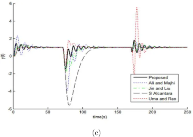
Time response associated with each of the considered methods is shown in Figure 9(a). The su-periority of the proposed method in servo tracking and disturbance rejection is obvious. The control input signals are shown in Figure 9(b), where, the methods of Jin, Uma and Alcantara require larg-er control inputs, compared with the method proposed in this research. The proposed method pro-vides a good set-point tracking with moderate input usage together with a good disturbance rejec-tion.
In order to assess the robustness of various studied methods, a +40% perturbation in the time delay is considered, and the corresponding time responses are shown in Figure 9(c). This figure clearly depicts the far superior performance of the proposed method.
(a)
(c)
Figure 9: Time response (a) and control input (b) for rejection of disturbances
v
1 andv
2, in Example 4. Also, the time response to a unit set-point and step disturbances with +40% increase in is shown (c).5 EXPERIMENTAL VERIFICATION
This section deals with theoretical analysis and experimental studies of an AC servo motor in the real time. Use has been made of the Modbus RTU protocol for communication between the control-ler (a PC) and the motor driver.The schematic of the experimental setup is shown in Figure 10 where
and
'are two variable communication time delays, in the range of 30-400 mili-seconds. In order to make the problem more challenging, a fictitious time delay ( ) and an integrator term ( , , )were incorporated in the real-time. In section 5.1 i=0 and 3, and in section 5.2 i=1 and 3 are chosen. The Servo motor has the specification given in Table 2.Figure 10: flow diagram in Matlab/Simulink,
and
' are variablecommunication delays and is an add artificial delay.
Model BONMET - SA3LO6B
Input voltage AC 3 phases, 50/60 HZ, 200-230 V Output voltage AC 3 phases, 0-230 V
Smps 6 A
In the first step, the transfer function of the servo motor was identified experimentally, by ap-plying a random input voltage to the servo motor, and measuring the velocity, and analyzing the results using the MATLAB identification toolbox, with 83 % fitness index, as given below:
864.7907) 395.5641
92.8620 8.1993
(
859.8850
= 4 3 2
s s
s s
s
e s
P i
s
(30)
where, =0 and i=0.
In order to evaluate the effectiveness of the proposed control method for FOPTD and IFOPTD plants, two experimental studies were considered as follows.
5.1 Plant Modeled as FOPTD
For i=0 and 0 in 30 and using (Steadman andHymas, 1979), the plant given by (30) can be formed as follows
1 0.156
= (0.356 )
s e s G
s
which is in the form of (2). The proposed controllers should be in the form of (8) and (9), for which the required parameters are found from Table 1. In particular, for =0and =3, the values of
0.217 = d
k and =0.133are obtained.
Time responses to a unity step commandand disturbance changes are obtained from simulation, as well as, experimental implementation, and the results are shown in Figure 11. Results show an exceptional similarity between the simulation and experimental results, while both have desirable closed loop performance and robustness.
Figure 11:Comparison between simulation and experimental results, by modeling the plant as an FOPTD system.
5.2 Plant Modeled as IFOPTD
( )
3.3.
s
e
G s
s
s
-+
The proposed controllers are in the form of (16) and (17), for which the required parameters are very simple to find from Table 1. In particular, for
=0, the values of ki=0.157, kd =0.217and =0.133 are obtained.
By using table 1 and for =3 and
=0, valueski =0.157, kd=0.217, and =0.1324 are obtained.Time responses to a unity step command and disturbance changes are obtained from simula-tion, as well as, experimental implementasimula-tion, and the results are shown in Figure 12. Once again, the results show an exceptional similarity between the simulation and experimental results, while both have desirable closed loop performance and robustness.
Figure 12: Comparison between simulation and experimental results, by modeling the plant as an IFOPTD system.
6 CONCLUSIONS
In this paper a new and simple method for control of stable and integrating systems with time de-lay was proposed. The controller design process includes designing unknown gains, for which very simple tuning formulae were proposed. The controller design process was studied in through simula-tion studies and comparison with some recent methods proposed in the literature. Based on the implemented studies, the proposed method was shown to have a very good performance in terms of the input tracking, disturbances rejectionand robustness against uncertainty in the time delay, and control input requirements, as compared to the five other methods proposed in the literature. The results of simulations revealed that some of the recently introduced methods need an excessive in-put usage to preserve the disturbance rejection property of the closed-loop, and hence, they may not be efficient methods from practical point of view.
References
Alcntara, S., Vilanova, R., Pedret, C., (2013). PID control in terms of robustness/performance and servo/regulator trade-offs: A unifying approach to balanced autotuning. Journal of Process Control, 23(4), 527-542.
Alfaro, V. M., Vilanova, R., (2012). Robust tuning and performance analysis of 2DoF PI controllers for integrating controlled processes. Industrial & Engineering Chemistry Research, 51(40), 13182-13194.
Ali, A., Majhi, S., (2010). PID controller tuning for integrating processes. ISA transactions, 49(1), 70-78.
Astrom, K. J and T. Hgglund., (1995). PID controllers: theory, design, and tuning. Instrument Society of America, Research Triangle Park, NC.
Astrom,K. J., Panagopoulos, H., Hgglund, T., (1998). Design of PI controllers based on non-convex optimization. Automatica, 34(5), 585-601.
Cvejn, J., (2013). The design of PID controller for non-oscillating time-delayed plants with guaranteed stability margin based on the modulus optimum criterion. Journal of Process Control, 23(4), 570-584.
Garca, P., and Albertos, P., (2013). Robust tuning of a generalized predictor-based controller for integrating and unstable systems with long time-delay. Journal of Process Control, 23(8), 1205-1216.
Garca, P., and Albertos, P., (2008). A new dead-time compensator to control stable and integrating processes with long dead-time. Automatica, 44(4), 1062-1071.
Hang, C. C., Wang, Q. G., and Yang, X. P., (2003). A modified Smith predictor for a process with an integrator and long dead time.Industrial and engineering chemistry research, 42(3), 484-489.
Jin, Q. B., Liu, Q., (2014). Analytical IMC-PID design in terms of performance/robustness tradeoff for integrating processes: From 2-Dof to 1-Dof. Journal of Process Control, 24(3), 22-32.
Kaya, I., (2003). Obtaining controller parameters for a new PI-PD Smith predictor using autotuning. Journal of Process Control, 13(5), 465-472.
Kwak, H. J., Sung, S.W., Lee, I.B., (2001). Modified Smith predictors for integrating processes: Comparisons and proposition.Industrial and engineering chemistry research, 40(6), 1500-1506.
Liu, T., Gao, F., (2011). Enhanced IMC design of load disturbance rejection for integrating and unstable processes with slow dynamics.ISA transactions, 50(2), 239-248.
Majhi, S., & Atherton, D.P., (2000). Obtaining controller parameters for a new Smith predictor using autotun-ing.Automatica, 36(11), 1651-1658.
Matauek, M.R., (1996). A modied Smith predictor for controlling a process with an integrator and long dead-time. Automatic Control, IEEE Transactions on, 41(8), 1199-1203.
Matauek, M.R., Ribi, A. I., (2012). Control of stable, integrating and unstable processes by the Modi ed Smith Pre-dictor. Journal of Process Control, 22(1), 338-343.
Normey-Rico, J. E., Camacho, E. F., (2009). Unified approach for robust dead-time compensator design. Journal of Process Control, 19(1), 38-47.
Shamsuzzoha, M., Lee, M., (2007). IMC-PID controller design for improved disturbance rejection of time-delayed processes. Industrial & Engineering Chemistry Research, 46(7), 2077-2091.
Shamsuzzoha, M., Lee, M., (2008). Analytical design of enhanced PID filter controller for integrating and first order unstable processes with time delay. Chemical Engineering Science, 63(10), 2717-2731.
Shamsuzzoha, M., Skogestad, S., (2010). The setpoint overshoot method: A simple and fast closed-loop approach for PID tuning. Journal of Process Control, 20(10), 1220-1234.
Skogestad, S., (2003). Simple analytic rules for model reduction and PID controller tuning.Journal of process control, 13(4), 291-309.
Steadman, J.F., Hymas, D.L., (1979). Evaluation of the Sundaresan Krishnaswamy technique for identification and control of multi capacity processes. The Canadian Journal of Chemical Engineering, 57(3), 381-382.
Tan, W., Marquez, H. J., Chen, T., (2003). IMC design for unstable processes with time delays. Journal of Process Control, 13(3), 203-213.
Torrico, B.C., Normey-Rico, J. E., (2005). 2DOF discrete dead-time compensator for stable and integrative process-es with dead-time. Journal of Procprocess-ess Control, 15(3), 341-352.
Uma, S., Rao, A. S., (2014). Enhanced modified Smith predictor for second-order non-minimum phase unstable processes. International Journal of Systems Science, (ahead-of-print), 1-16.
Vanavil, B., Chaitanya, K.K., Rao, A.S., (2015). Improved PID controller design for unstable time delay processes based on direct synthesis method and maximum sensitivity. International Journal of Systems Science, 46(8), 1349-1366.
Wang, Q. G., Hang, C. C., Yang, X. P., (2001). Single-loop controller design via IMC principles. Automatica, 37(12), 2041-2048.
Zhang, W., Rieber, J. M., Gu, D., (2008). Optimal dead-time compensator design for stable and integrating processes with time delay. Journal of Process Control, 18(5), 449-457.