Abstract—Space-frequency DORT (SF-DORT) is an effective time-reversal (TR) imaging method due to its immunity to the noise and adaptability of complex environment. However, some potential drawbacks, such as low range and co-range resolutions, make SF-DORT inferior to the Space-frequency MUSIC (SF-MUSIC). In this paper, we propose a novel high-resolution imaging method utilizing SF-DORT combining an extrapolated virtual array (EA-SF-DORT). The virtual extrapolated TR array is created by autoregressive vector extrapolation (ARVE). In this way, the aperture of the TR array is extended significantly and the drawbacks associated with SF-DORT can be improved. Simulation results demonstrate that SF-DORT combining the extrapolated virtual array achieve much higher range and co-range resolutions than conventional SF-DORT.
Index Terms—Time-reversal (TR) imaging, the decomposition of the time-reversal operator (DORT),Space-frequency DORT (SF-DORT), Extrapolated array, Autoregressive vector extrapolation (ARVE).
I. INTRODUCTION
Time reversal (TR) technique has attracted enormous attention in radar imaging fields in recent
years due to its spatial and temporal high-resolution focusing characteristics [1]. The TR operator
(TRO) is one of the most fundamental TR imaging method, and TRO form the basis of the
decomposition of the time-reversal operator (DORT) and the TR multiple signal classification
(TR-MUSIC) [2]-[4]. Space-frequency decomposition of the time-reversal operator (SF-DORT) and SF
multiple signal classification (SF-MUSIC) are faster TR imaging methods because they obtain the
multistatic data matrices (MDMs) much more conveniently than DORT and TR-MUSIC [5]-[8].
Although SF-DORT works well under increased clutter and noise levels, its range and co-range
resolutions are inferior to SF-MUSIC [9].
To overcome the shortcomings of SF-DORT, utilizing virtual extrapolated array is a promising
solution because it is suitable for an array with limited aperture and meets the requirement of
miniaturizing the imaging system [10]. The autoregressive vector extrapolation (ARVE) [11], which
exploits the spatial-temporal coupling of the matrix constituted by the received signals, predicts the
signals on the virtual antennas more accurately than the 1-D AR extrapolation in [12]-[13].
Based on the above analysis, we propose a novel high-resolution imaging method utilizing
SF-High-Resolution Imaging Utilizing
Space-Frequency DORT Combining
the Extrapolated Virtual Array
1
Qiang Du, 1Yaoliang Song , 1Tong Mu, 1Zeeshan Ahmad
School of electronic and optical engineering, Nanjing University of science and technology, Nanjing, China
DORT combining the virtual extrapolated array (EA-SF-DORT) in this article. The performance
deterioration of imaging caused by applying the ARVE with the noise matrix can be offset by
SF-DORT, and high-resolution can be achieved. Simulations show that SF-DORT utilizing the
extrapolated virtual array can achieve much higher range and co-range resolutions than without
utilizing.
The rest of this paper is organized as follows. Section II shows the whole processing chain of the
proposed TR imaging method, including the principle of ARVE and SF-DORT. To illustrate the
high-resolution imaging capability, computer simulations are conducted, and the results are given in
Section III. Finally, Section IV offers some conclusions drawn on the basis of simulation results.
II. THE PRINCIPLE OF PROPOSED TR IMAGING METHOD
The processing chain of this novel method is shown in Fig. 1 and could be divided into two stages.
In the first stage, the matrix constituted by the received noised-signals, or called the original
measurement data set, S, is extrapolated by ARVE. Afterwards, the SF-DORT has been applied to the
extrapolated matrix SE and high-resolution targets imaging has been achieved.
Original Measurement
data setS
Stage 1 ARVE on
Stage 2 SF-DORT on SE
S
E S
Output: TR imaging
Fig. 1. The processing chain of the new TR imaging method.
A. The principle of ARVE
Assume a TR array, which contains L real antennas, lies parallel to the x-axis. Assume the TR array
receives the same linear frequency modulated (LFM) signals, so the received signals are coherent.
The received signal on the l-th real antenna is given below
1
( ) ( , ) ( ) ( )
s
M
ml
l l
m t n f
s n s l n s t n t c
, (1)where ml is the distance from the m-th target to the l-th antenna. m is the target index and
1, 2, ,
m M. All the targets are located in the far field. l is the antenna index and l1, 2, ,L. n is the temporal sampling index andn0,1, ,N. fs is the sampling rate. n tl( ) is the noise on the l-th antenna. s(t) is the LFM signal and can be expressed as follow
2 0
1
( ) cos(2 ( ( )- ))
2
s t f t t , (2)
where
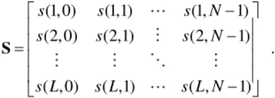
B t/ 0, B is the signal bandwidth, t0 is the duration of the signalt0N fs and f0 is thestarting frequency. So the centre frequency of the LFM signal is f0B 2. Over N measurements, we
(1,0) (1,1) (1, 1)
(2,0) (2,1) (2, 1)
( ,0) ( ,1) ( , 1)
s s s N
s s s N
s L s L s L N
S . (3)
With the original measurement data S in hand, the extrapolated data SE is formulated through ARVE. The principle of ARVE is shown in Fig. 2 and can be divided into three steps.
Original measurement
data set S
Stage 1: ARVE on
Step 1 Select the Order of
the AR Model Algoriths:Typical
ranges, MDL
Step 2 Estimate the block AR
model parameters Algoriths: 2-D Lattice
linear prediction parameter estimation
Step 3 Vector extrapolation
Col. Vector
Col. Vector
Rows Forwards
Rows Backwards
Column Rows
S
Output: Extrapolated
data set
U
E
D
=
S
S S
S
Fig. 2. Virtual measurement data are created by modeling the original measurements with a 2-D AR model and then using vector extrapolation
The first step is to determine the number of parameters of S, i.e. select the order of the AR model.
The number of parameters is denoted by a pair ( p1, p2), where p1 is the order of the spatial
dimension and p2 is the order of the temporal dimension. Both p1 and p2 are positive integers and
can be determined by S itself. This step can be done by choosing the typical value of the model order
directly or using an order estimation algorithm such as MDL [14]. The typical range for p1 is
between 1 and L 2. The typical range for p2 is between 1 and N 2. The pair (1, 1) should be
excluded [10].
With the number of parameters determined, the next step is estimating the block AR model
parameters. We will adopt the approach 2-D lattice linear prediction parameter estimation in [15]
In the last stage, we provide a brief summary of the vector extrapolation equations. Given a column
vector of size(p2 1) 1as follows
2( ,1 2) ( ,1 2) ( ,1 2 1) ( ,1 2 2)
T
p n n s n n s n n s n n p
s , (4)
and the forward linear vector extrapolation is given in (5)
1
2 1 2 2 2 1 2
1
ˆ ( , ) ( ) ( , )
p F
p p p
i
n n i n i n
s A s , (5)
where
2 1 2
ˆFp ( ,n n )
s is the virtual measurement vector of size(p2 1) 1, and the superscript F represents
forward. 2( )
p i
A is the i-th block of the AR parameters in (5) and of size (p2 1) (p21).
The backward linear vector extrapolation is given by
1
2 2 2 2 2
*
1 1 2 1 1 2
1
ˆ ( , ) ( ( ) ) ( , )
p B
p p p p p
i
n p n i n p i n
s J A J s , (6)
where * represents the conjugate operation. 2 p
J is a reflection matrix of dimension(p2 1) (p21)
whose anti-diagonal elements are one and all other elements are zero, i.e.,
2
0 0 1
0 0
0 1 0
1 0 0
p
J . (7)
For more details about vector extrapolation equations, please see [7] and [11].
Therefore, the matrix S can be extrapolated to the matrix SE as follows:
1 1 1
2 2 2
(0) (1) ( 1)
(0) (1) ( 1)
(0) (1) ( 1)
L L L
g g g N
g g g N
g g g N U E D S S S S
, (8)
where
1 1 1 ( 1) / 2 1 ( 1) / 2 1 ( 1) / 2 1
2 2 2 ( 1) / 2 2 ( 1) / 2 1 ( 1) / 2 2
( 1) / 2 ( 1) / 2 ( 1)
(0) (1) ( 1) (0) (1) ( 1)
(0) (1) ( 1) (0) (1) ( 1)
(0) (1) ( 1) (0) (1)
L L L
L L L
L L L L L L
s s s N g g g N
s s s N g g g N
s s s N g g g
S
/ 2(N 1)
.
is the spatial extrapolation factor of the array. The original data set S is the central part of SE. SUand D
S are extended data from the top and bottom of the matrix Srespectively.
B. TR imaging based on SF-DORT
1 1 1 2 1
2 1 2 2 2
1 2
( ) ( ) ( )
( ) ( ) ( )
( ) ( ) ( )
N
N
L L L N
k k k
k k k
k k k
K . (9)
Appling SVD to K, we have
K UΛV (10)
where Λ is a N × M real diagonal matrix which contains singular values. U is an N × N unitary matrix,
and V is the M × M matrix. Since the matrix K includes the spatial and frequency of the target,
applying SVD to K is called SF decomposition. Assume Up as the p-th column of the matrix U, Vp
as the p-th column of the matrix V, and p as the p-th singular value. Up contains the spatial
relationships between the p-th target and the extrapolated array while Vprepresents the frequency
content of the received signals. Assuming S(ω) as the Fourier transform of the transmitted signal s(t),
a new N × 1 retransmitted vector function can be defined as below
T TR( ) pS( ) U Sp,1 ( ) Up,2S( ) Up,LS( )
R U , (11)
where Up Up,1 Up,2 Up,LTand "T" denotes transposition. By applying inverse Fourier
transform to each row of RTR( )
, we could get the time-domain TR signal rTR( )t .Once the vector RTR( )
or rTR( )t is obtained, we can get the following pseudo-spectrum I P( s) at the search point PS in the spatial domain.s s TR 0 s TR
( ) ( , ), ( ) ( , ) ( )
t
t t d
I P g P r G P R , (12)
where G P( , )s
is the Fourier transform of g P( , )s t . N 1.G P( , )s
is the background Green’s function vector at the search point PS ( , )x y to focus the target and is given by
Ts s 1 s 2 s
( , ) G( , , ) G( , , ) G( , N, )
G P P R P R P R (13)
with G( ,P Rs 1, ) is the background Green’s function in free space, and Rn(n1, 2, , )N is the locations of the n-th antenna.
III. SIMULATIONS
In this section, we compare the range and co-range resolutions utilizing conventional SF-DORT and
the proposed EA-SF-DORT for two different cases. The first is a single target case while the second is
the multi-target one. We utilize SF-DORT to evaluate the targets detection performance.
The linear TR array is shown in Fig. 3. It contains 4 real antennas and 12 virtual antennas, so L=4
and the extrapolation factor α=4. All the antennas lie parallel to the x-axis. The distance between the
adjacent antennas is set as d and d is 0.075m. The four real antennas are located at (50m, 0.25m),
are located at (49.55m, 0.25m), (49.625m, 0.25m), (49.7m, 0.25m), (49.775m, 0.25m), (49.85m,
0.25m), (49.925m, 0.25m) and (50.3m, 0.25m), (50.375m, 0.25m), (50.45m, 0.25m), (50.525m,
0.25m), (50.6m, 0.25m), (50.675m, 0.25m) respectively.
The received LFM signal can be expressed in (2). The parameters of the LFM signal are as follows:
B=0.5GHz, N=4000, fs4.5GHz, f02.25GHz. The signal to noise ratio (SNR) is 10 dB.
x(m) y(m)
target
v1 v2 v3 v4 v5 v6 r7 r8 r9 r10 v11 v12 v13 v14 v15 v16
Fig. 3. Ilustration of the TR array placed parallel to the x-axis and the target in the far field, “v” denotes virtual antennas and “r” denotes real antennas.
A. Imaging for a single target case
Consider the single point target located at (62.5m, 75m). All the antennas in the TR array receives
LFM signal.
The range and co-range resolutions given by SF-DORT with and without autoregressive vector
extrapolation are shown in Fig 4. It can be observed that the peak appear at the target location with
and without extrapolation, but the sidelobes are much lower and the mainlobe is much narrower when
extrapolation is used. The raising in co-range resolution is superior to the raising in range resolution
because the co-range resolution is inversely proportional to the effective aperture of the array and the
proposed extrapolation method increases the aperture effectively.
(a)
0 20 40 60 80 100
-80 -70 -60 -50 -40 -30 -20 -10 0
x(m)
dB
(b)
Fig. 4. Range and co-range resolutions utilizing SF-DORT and EA-SF-DORT for a single target and the target is located
at (62.5m,75m) (a) Co-range resolutions (b) Range resolutions
B. Imaging for a multi-target case
In this simulation, we consider a two targets case when the targets are located at (75m,62.5m) and
(25m, 37.5m) respectively. All the antennas in the TR array receive the same LFM signal. The
extrapolation factor α is 4 and the extrapolated matrix SE has the size of (16×4000). Once the left singular vectorsUp, p = 1, . . . , P , P = 2 have been acquired using (10), we could locate the two
targets with the same procedure above.
The comparison of range and co-range resolutions for the target located at (75m, 62.5m) given by
SF-DORT with and without ARVE are shown in Fig. 5, while the same comparison for the target
located at (25m, 37.5m) are shown in Fig. 6. From Fig. 5 and Fig. 6 the range and co-range
resolutions are much higher when extrapolation is used, especially the range resolution for the target
at (25m, 37.5m).
(a)
0 20 40 60 80 100
-120 -100 -80 -60 -40 -20 0
y(m)
dB
Conventional SF-DORT EA-SF-DORT, α=4 Target Location
0 20 40 60 80 100
-140 -120 -100 -80 -60 -40 -20 0
x(m)
dB
(b)
Fig. 5. Range and co-range resolutions utilizing SF-DORT and EA-SF-DORT for Multitargets case, the target is located
at (75m,62.5m). (a) Co-range resolutions (b) Range resolutions
(a)
(b)
Fig. 6. Range and co-range resolutions utilizing SF-DORT and EA-SF-DORT for Multitargets case, the target is located
at (25m,37.5m). (a) Co-range resolutions (b) Range resolutions
0 20 40 60 80 100
-150 -100 -50 0
y(m)
dB
Conventional SF-DORT EA-SF-DORT, α=4 Target Location
0 20 40 60 80 100
-140 -120 -100 -80 -60 -40 -20 0
x(m)
dB
Conventional SF-DORT EA-SF-DORT, α=4 Target Location
0 20 40 60 80 100
-140 -120 -100 -80 -60 -40 -20 0
y(m)
dB
IV. CONCLUSION
In this paper, we have presented a novel high-resolution TR imaging method utilizing SF-DORT
combining virtual array created by ARVE (EA-SF-DORT). The ARVE extends the aperture of the TR
array significantly, consequently overcomes the shortcomings of conventional SF-DORT. It has been
shown that the SF-DORT utilizing extrapolated virtual array achieves much higher range and
co-range resolutions than conventional SF-DORT. Simulation results validate the satisfying performance
of the proposed method.
ACKNOWLEDGMENT
This work is sponsored by the National Natural Science Foundation of China under grant
No.61571229 and 61271331.
REFERENCES
[1] Mathias Fink and Claire Prada. “Acoustic time-reversal mirrors”,Inverse Probl.,Vol.17, No.3, pp. R1-R38, Feb. 2001. DOI: 10.1088/0266-5611/17/1/201.
[2] G. Micolau, M. Saillard. “D.O.R.T. method as applied to electromagnetic subsurface sensing”, Radio Sci., vol. 38,no. 3, pp. 4-1 - 4-12, Jun. 2003. DOI: 10.1029/2000RS002590.
[3] Mehmet E. Yavuz, Fernando L. Teixeira. “Full time-domain DORT for ultrawideband electromagnetic fields in dispersive, random inhomogeneous media”, IEEE Trans. Antennas Propag., vol. 54, no. 8, pp. 2305-2315, Aug. 2006. DOI: 10.1109/TAP.2006.879196. [4] X.M. Zhong, C. Liao, W.B. Lin, H.Y. Li and H.J. Zhou. “Time-reversal imaging based on the space-frequency MDM and cancellation
operator”, J. Electromagn. Waves Appl. s,Vol.28, No.3, pp. 265-274, Feb. 2014. DOI: 10.1080/09205071.2013.861751 [5] Xuanming Zhong, Cheng Liao, and Wenbin Lin. “Space-Frequency Decomposition and Time-Reversal Imaging”,IEEE Trans.
Antennas Propag.,Vol.63, No.12, pp. 5619-5628, Dec. 2015. DOI: 10.1109/TAP.2015.2490579.
[6] Xuanming Zhong, Cheng Liao, and JuFeng. “Time-reversal time-domain imaging algorithm based on space-frequency decomposition”,
Chin. J. Radio Sci.,Vol.29, No.3, pp. 476-479, Jun. 2014.
[7] Mehmet E. Yavuz, Fernando L. Teixeira. “Space–Frequency Ultrawideband Time-Reversal Imaging”, IEEE Trans. Geosci. Remote
Sens., vol. 46, no. 4, pp. 1115-1124, Mar. 2008. DOI: 10.1109/TGRS.2008.915755.
[8] M. E. Yavuz, A. E. Fouda, and F. L. Teixeira. “GPR Signal Enhancement Using Sliding-Window Space-Frequency Matrices”, Prog. Electromagn. Res., vol. 45, no. 4, pp. 1-10, 2014.
[9] Javad Ebrahimi-Zadeh, Mojtaba Dehmollaian, and Karim Mohammadpour-Aghdam. “Electromagnetic Time-Reversal Imaging of Pinholes in Pipes”, IEEE Trans. Antennas Propag., Vol.64, No.4, pp.1356-1363, Apr. 2016. DOI: 10.1109/TAP.2016.2526043. [10] C. S. Marino and P. M. Chau. “Constrained Sensor System Resolves Closely Spaced Obscured Low-SNR Sources Using Virtual
Beamforming”, IEEE Trans. Instrum. Meas., vol. 63, no. 1, pp. 231-242, Jan 2014. DOI: 10.1109/TIM.2013.2275239.
[11] C. S. Marino and P. M. Chau, “Low-Level Sinusoidal Signal Detection From a High-Resolution Virtual Spectral Image Using Autoregressive Vector Extrapolation,” IEEE Trans. Instrum. Meas., vol. 61, no. 9,pp. 2413–2421, Sep. 2012. DOI: 10.1109/TIM.2012.2190549.
[12] F. Wan, W.-P. Zhu, and M. N. S. Swamy, “Spacial Extrapolation-Based Blind DOA Estimation Approach for Closely Spaced Sources”, IEEE Trans.Aerosp. Electron. Syst., vol. 46, no. 2, pp. 569–582, Apr. 2010. DOI: 10.1109/TAES.2010.5461642.
[13] C. S. Marino and P. M. Chau : “High resolution full aperture processing of data limited scenarios through synthetically extending the temporal data”, Proc. 39th Asilomar Conf. on Signals, Syst. Comput., Pacific Grove, CA, USA, 2005, pp.1394-1398.
[14] S. L. Marple, Jr., Digital Spectral Analysis. Englewood Cliffs, NJ, USA: Prentice-Hall, 1987.