Nulls and Side lobe Levels Control in a
Time Modulated Linear Antenna Array
by
Optimizing Excitations and Element
Locations Using RGA
Bipul Goswami and Durbadal Mandal
Department of Electronics and Communication Engineering National Institute of Technology Durgapur
West Bengal, India- 713209
Email: {durbadal.bittu, goswamibipul}@gmail.com
Abstract—In this paper a novel approach based on the Real coded Genetic Algorithm (RGA) is proposed to improve nulling performance as well as suppression of Side Lobe Level (SLL) of a Time Modulated Linear Antenna Arrays (TMLA). RGA adjusts the static excitation amplitudes as well as the location of each element from the origin to place deeper nulls in the desired direction. Three design examples are presented that illustrate the use of the RGA, and the optimization goal in each example is easily achieved.
Index terms — Time Modulated Linear Antenna Array; Far-field Pattern; Genetic Algorithm; Amplitude Excitation; Deeper Null; Side Lobe Level.
I. INTRODUCTION
Antenna Array is formed by assembling the radiating elements in a particular electrical or geometrical configuration. In most cases the elements are identical. Total field of the antenna array is found by vector addition of the fields radiated by each individual element. There are five control parameters in an antenna array that can be used to shape the pattern properly, they are, the geometrical configuration (linear, circular, rectangular, spherical etc.) of the overall array, relative displacement between elements, excitation amplitude of the individual elements, excitation phase of the individual elements and relative pattern of the individual elements [1-4]. In many communication applications it is required to design a highly directional antenna. Antenna Arrays have high gain and directivity compared to an individual radiating element.
As compared to conventional antenna arrays, the time modulated antenna arrays introduce a fourth
sideband signals spaced at multiples of modulation frequency, which implies that part of electromagnetic energy radiated or received by the antenna array was shifted to the sidebands.
The increasing pollution of electromagnetic environment has prompted the study of array pattern nulling techniques. These techniques are very important in radar, sonar and communication systems for minimizing degradation in signal to noise ratio performance due to undesired interference [3-4]. A lot of research works are going on for reducing the signal at nulls and Side Lobe Levels [5-20]. Time modulated antenna arrays are attractive for the synthesis of low/ultralow side lobes [6–7, 11-13]. In [6-7, 11], a differential evolution algorithm has been used to optimize the static-mode coefficients as well as the durations of the time pulses leading to a significant reduction of the sideband level. An approach to induce deeper nulls by controlling excitations amplitude of antenna elements in a time modulated array using Genetic Algorithm has been proposed in [8]. An approach for estimating direction of arrivals (DOA) in TMLAs with unidirectional phase center motion (UPCM) scheme is proposed in [9].
Design goal of this paper is to introduce deeper null/nulls to some desired direction and to suppress the relative SLL with respect to main beam for a TMLA of isotropic elements. This is done by designing the relative spacing between the elements, with a non-uniform excitation over the array aperture. This involves non-monotonic variation in antenna element parameters, which becomes a highly complex optimization problem. The classical optimization methods cannot bear the demand of such complex optimization problem.
Classical optimization methods have several disadvantages such as: i) highly sensitive to starting points when the number of solution variables and hence the size of the solution space increase, ii) frequent convergence to local optimum solution or divergence or revisiting the same suboptimal solution, iii) requirement of continuous and differentiable objective cost function (gradient search methods), iv) requirement of the piecewise linear cost approximation (linear programming), and v) problem of convergence and algorithm complexity (non-linear programming). For the optimization of such complex, highly non-linear, discontinuous, and non-differentiable array factors; various heuristic search evolutionary techniques were adopted. In this paper, the evolutionary technique, Real coded Genetic Algorithm (RGA) [3-4, 21-23] is used to get the desired pattern of the array. The time modulation period is divided into numerous minimal time steps with the same length, where the ON-OFF status for each time step is followed by a scheme given in the paper.
The rest of the paper is arranged as follows: in section II, the general design equations for the non-uniformly excited and unequally spaced linear antenna array are stated. Then, in section III, a brief introduction for the Genetic Algorithm is presented. Numerical simulation results are presented in section IV. Finally the paper concludes with a summary of the work in section V.
II. DESIGN EQUATIONS
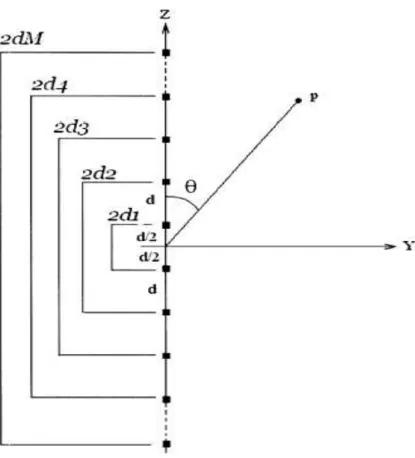
A broadside linear array of 2M isotropic radiators [1-2] is considered as shown in Figure 1, in which each element is controlled by a high speed RF switch and excited with non uniform current excitation. The array elements are assumed to be uncoupled and having equal inter-elements spacing along the z-axis with its centre at the origin. The array is symmetric in both, geometry and excitation with respect to the array centre. Only Amplitude excitations and spacing between each element are used to change the antenna pattern.
Fig. 1. Geometry of a 2M element symmetric linear array along the z axis.
The free space far-field pattern [1-2] in azimuth plane (x-y plane) with symmetric amplitude distributions is given by (1):
n n
n M
n
n t I kX U
t d I
AF
)
cos(
cos
)
(
2
)
,
,
,
(
1
where,
denotes the angle measured from the broadside direction of the array. In,
nand Xn are respectively, current excitation amplitude, excitation phase, and location of the nth element from the origin. In this paper
n is kept as zero. k
2
, the propagation constant where
being thesignal wave length, d is the spacing between elements, 2M is total number of elements in the array.
)
(
tUn =periodic switch ON-OFF time sequences function for n th
where each element is switched ON for
, where 0 ≤
≤ T.The array elements are numbered 1 to M from the origin in a symmetric array where total numbers of
elements are 2M. Firstly the left most P elements (P < M) are turned on for time step τ, where
1
P M T
(2)Here T is the time modulation period. In first time step, the P consecutive elements numbered from 1 to P are switched ON. In the next time step, 2 to P+ 1 are switched ON and so on. In this work
)
(
tUn is taken as [6-7]:
other wise t t Un
1 2,
,
0
1
)
(
(3)where other wise P n P n
,
,
0
1
(4)otherwise P M n P M n
1
,
,
1
2
(5)
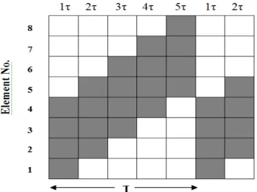
Fig. 2. Switch on time sequences of a 16 element (M=8) TMLA with P=4.
After defining the far-field radiation pattern, the next step in the design process is to formulate the objective function which is to be minimized.The objective function “Cost Function” (CF) or Fitness function which to be minimized with RGA for introducing deeper null is given in (6).
Kk
k m
i
i
Q k H C
AF null AF
C CF
1 2 max
1
1
(
)
(
)
)
(
(6)Where m is the maximum number of positions where null can be imposed. In this paper, one and two
has been considered as the value of ‘m’. AF
(
nulli)
is the array factor value at the particular null position. AFmax is the maximum value of the array factor. The second term in the CF is added to reduce the side lobe up to a desired level. Here K denotes number of side lobes in the original pattern.k
Q is the side lobe level in dB generated by the individual population at some peak point
k.
is the desired value of the side lobe level in dB. H(k) is defined as
0
)
(
0
)
(
,
,
0
1
k k Q Q k
H (7)
The side lobes whose peak exceeds threshold
, that side lobe must be suppressed and for this purpose H(k) is adopted in the “cost function” expression. In cost function, for the first term, both the numerator and denominator are absolute. Further C1 and C2 are the weighting factors. The weight C1 and C2III. EVOLUTIONARY TECHNIQUE: REAL-CODED GENETIC ALGORITHM
GA is mainly a probabilistic search technique, based on the principles of natural selection and evolution. At each generation it maintains a population of individuals where each individual is a coded form of a possible solution of the problem at hand and called chromosome. Chromosomes are
constructed over some particular alphabet, e.g., the binary alphabet {0, 1}, so that chromosomes’
values are uniquely mapped onto the decision variable domain. Each chromosome is evaluated by a function known as fitness function, which is usually the fitness function or the objective function of the corresponding optimization problem.
Steps of RGA as implemented for optimization of spacing between the elements and current excitations are [3-4], [18-20]:
Initialization of real chromosome strings of np population, each consisting of a set of
excitations. Size of the set depends on the number of excitation elements in a particular array design.
Decoding of strings and evaluation of CF of each string.
Selection of elite strings in order of increasing CF values from the minimum value. Copying of the elite strings over the non-selected strings.
Crossover and mutation to generate off-springs. Genetic cycle updating.
The iteration stops when the maximum number of cycles is reached. The grand minimum CF and its corresponding chromosome string or the desired solution are finally obtained.
Fig. 3. The GA flow for determining the optimized excitation amplitude and optimum location of array elements.
Desired pattern is generated by jointly optimizing amplitude distributions and location of array elements from the array centre. Here, both excitation amplitude and element location distributions are assumed symmetric with respect to the centre of the array. The chromosomes are corresponded to current excitation weights of antenna elements and location of individual elements from the array centre. Because of symmetry, each chromosome consists of 2M number of genes where M is the number of antenna elements on either side of array centre. Here 1st to Mth genes represent current excitation weights of antenna elements and
(
M
1
)
thto2
Mth genes represent optimal elementlocations from the array centre. As an example chromosome one W1can be represented by (8).
W1
[
W11,
W12,....
W1M,
W1(M1),
W1(M2),...,
W1(2M)]
(8)Here, W11
,
W12,....
W1M are the antenna elements amplitude distributions and) 2 ( 1 ) 2 ( 1 ) 1 (
1M ,W M ,...,W M
current excitation weights and element locations has boundaries with upper and lower limit. The random set of chromosome can be easily constructed using following relation represented by (9). Wn
(
u1
u2)
r
u2 , u2
Wn
u1 (9)Where, u1 and u2 are the maximum and minimum limit value of the weights and r is real random vector between zero and one. RGA technique generates a set of normalized non-uniform current excitation weights and optimal spacing for all sets of time modulated linear antenna arrays.
IV. NUMERICAL RESULTS
A 12, 16, and 20 elements linear array of isotropic radiating elements, with λ/2 inter-element spacing, is considered for time modulated linear antenna array with T=16 s
.The required “switch-on” time intervals for each element can be calculated using (2). RGA is applied to get deeper nulls. Every time RGA executed with 400 iterations. The population size was fixed at 120. For the real coded GA, the mutation probability was set to 0.01 and uniform crossover with crossover probability 1 was taken. RGA algorithm is initialized using random values of excitation (
0
In
1
) and spacingbetween elements (
2
d
). For predefined nulls of the radiation pattern, the nulling performances are improved. Similarly at predefined peak positions, the nulls are imposed. The programming has been written in Matlab language using MATLAB 7.8.0(R2009a) version on core (TM) 2 duo processor, 3.00 GHz with 2 GB RAM.The Initial values of maximum SLL and Beam width between first nulls (BWFN) for uniform amplitude excitation (In
1
) and uniform spacing (
2
between adjacent elements) has been given in TABLE I.TABLEI.SLL AND BWFN FOR UNIFORM EXCITATION (In
1
) WITH
2
INTER-ELEMENTS SPACING LINEARARRAY
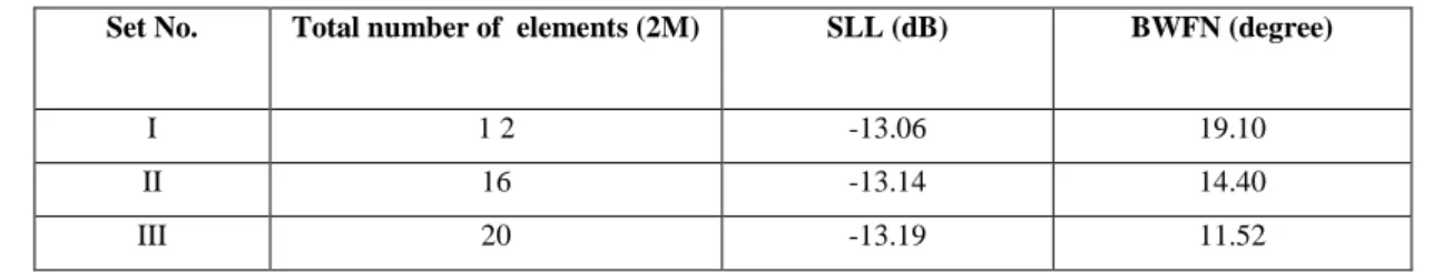
Set No. Total number of elements (2M) SLL (dB) BWFN (degree)
I 1 2 -13.06 19.10
II 16 -13.14 14.40
III 20 -13.19 11.52
M X X
X1
,
2,...,
are normalized using
2
. Figures 4-6 also depict the substantial reductions inmaximum peak of the SLL with non-uniform current excitation weights and optimal placement of array elements, as compared to the uniform current excitation weights (IM=1) and uniform inter-elements spacing (
2
between adjacent elements) case. For example, in optimized pattern the SLL is reduced by more than 1 dB from -13.06 dB down to -14.27 dB for 12 elements array. For 16 elements array in optimized pattern SLL is reduced by more than 1 dB from -13.14 dB down to –14.51 dB. For 20 elements array in optimized pattern SLL is reduced from -13.19 dB down to –14.22 dB. The improved values are shown in TABLE II and TABLE IIA.0 20 40 60 80 100 120 140 160 180
-80 -70 -60 -50 -40 -30 -20 -10 0
Angle of arival (degrees)
S
id
e
lo
b
e
le
v
el
(
d
B
)
In=1 & spacing: lamda/2 Optimized pattern
Fig. 4. Best array pattern found by GA for the 12-elements array case with an improved null at 3rd nulls i.e. = 600 and
= 1200.
0 20 40 60 80 100 120 140 160 180
-80 -70 -60 -50 -40 -30 -20 -10 0
Angle of arival (degrees)
S
id
e
l
o
b
e
l
e
v
e
l
(d
B
)
In=1 & spacing: lamda/2 GA Optimized Pattern
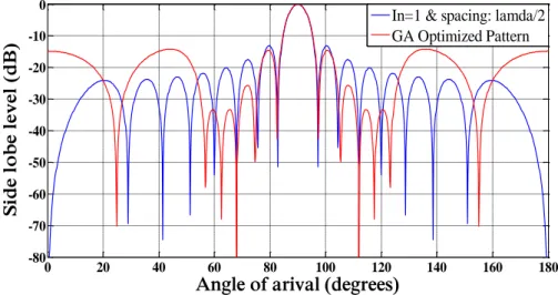
Fig. 5. Best array pattern found by GA for the 16-elements array case with an improved null at 3rd null i.e. = 680 and
0 20 40 60 80 100 120 140 160 180 -80
-70 -60 -50 -40 -30 -20 -10 0
Angle of arival (degrees)
S
id
e
l
o
b
e
l
e
v
e
l
(d
B
)
In=1 & spacing: lamda/2 GA Optimized Pattern
Fig. 6. Best array pattern found by GA for the 20-elements array case with an improved null at 3rd null i.e. = 72.500 and
= 107.500.
TABLE II. CURRENT EXCITATION WEIGHTS, INITIAL AND FINAL NULL DEPTH FOR NON-UNIFORMLY EXCITED TIME
MODULATED LINEAR ARRAY WITH OPTIMAL POSITION OF ELEMENTS (Xn) FROM ORIGIN FOR ONE NULL IMPOSED IN THE 3RD
NULL POSITION
No. of
Elements
M I I
I1
,
2,...,
;M X X
X1
,
2,....,
(Normalized with respect to 2 )Initial null
depth (dB)
Final null
depth (dB)
12 0.9903 0.6311 0.2147 0.2657 0.1023 0.0823; 0.5498
1.5952 2.6712 3.8133 4.9673 5.9893
-53.93 -92.04
16 0.9960 0.8629 0.1854 0.4579 0.2219 0.1788 0.1667
0.0557; 0.6064 1.7209 2.8607 3.9623 5.2483 6.3040
7.3990 8.5710
-50.60 -88.29
20 0.9278 0.9769 0.7940 0.2258 0.2171 0.3373 0.3796
0.2747 0.1890 0.2138; 0.5502 1.6514 2.6933 3.7407
4.9030 5.9060 6.9263 8.0007 9.1267 10.1433
-77.20 -90.00
TABLEIIA. SLL AND BWFN FOR NON-UNIFORMLY EXCITED TIME MODULATED LINEAR ARRAY WITH OPTIMAL SPACING
(Xn)FROM ARRAY CENTRE FOR ONE NULL IMPOSED AT 3RD
NULL POSITION.
No. of Elements SLL Final (dB) BWFN Final (degree)
12 -14.27 21.02
16 -14.51 14.40
20 -13.36 11.52
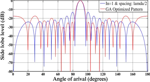
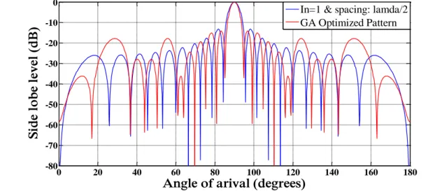
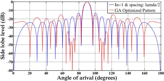
with initial values of -19.56 dB, -20.10 dB, -20.35 dB respectively. Figures 7-9 also depict the substantial reductions in maximum peak of the SLL with nonuniform current excitation weights and optimal placement of array elements, as compared to the uniform current excitation weights and uniform inter-elements spacing. For example, in optimized pattern the SLL is reduced by more than 1 dB from -13.06 dB down to -14.57 dB for 12 elements array. For 16 elements array in optimized pattern SLL is reduced by more than 4 dB from -13.14 dB down to –17.45 dB. For 20 elements array in optimized pattern SLL is reduced by more than 1 dB from -13.19 dB down to –14.22 dB. The improved values are shown in TABLE III and TABLE IIIA.
0 20 40 60 80 100 120 140 160 180
-80 -70 -60 -50 -40 -30 -20 -10 0
Angle of arival (degrees)
S
id
e
l
o
b
e
l
e
v
e
l
(d
B
)
In=1 & spacing: lamda/2 Optimized Pattern
Fig. 7. Best array pattern found by GA for the 12-elements array case with a null introduced at 3rd peak i.e. = 54.500 and
125.500.
0 20 40 60 80 100 120 140 160 180
-80 -70 -60 -50 -40 -30 -20 -10 0
Angle of arival (degrees)
S
id
e
l
o
b
e
l
e
v
e
l
(d
B
)
In=1 & spacing: lamda/2 GA Optimized Pattern
Fig. 8. Best array pattern found by GA for the 16-elements array case with a null introduced at 3rd peak i.e. = 64.400 and
.
0 20 40 60 80 100 120 140 160 180
-80 -70 -60 -50 -40 -30 -20 -10 0
Angle of arival (degrees)
S
id
e
lo
b
e
le
v
el
(
d
B
)
In=1 & spacing: lamda/2 GA Optimized Pattern
Fig. 9. Best array pattern found by GA for the 20-elements array case with a null introduced at 3rd peak i.e. = 69.700 and
=110.300.
TABLE III. CURRENT EXCITATION WEIGHTS,INITIAL PEAK AND FINAL NULL DEPTH FOR NON-UNIFORMLY EXCITED TIME
MODULATED LINEAR ARRAY WITH OPTIMAL POSITION OF ELEMENTS (Xn) FROM ORIGIN FOR ONE NULL IMPOSED IN THE
3RD
PEAK POSITION.
No. of
Elements
M I I
I1
,
2,...,
;M X X
X1
,
2,....,
(Normalized with respect to
2
)Initial Peak
depth (dB)
Final Null
depth (dB)
12 0.8596 0.4000 0.1975 0.1290 0.1447 0.1109; 0.5629
1.8224 2.9448 3.9963 5.0663 6.2200
-19.56 -79.60
16 0.8363 0.2757 0.4528 0.3001 0.2213 0.1470 0.1286
0.0387; 0.5786 1.6428 2.7752 3.9237 5.0387 6.2760
7.5177 8.6637
-20.10 -83.17
20 0.9278 0.9769 0.7940 0.2258 0.2171 0.3373 0.3796
0.2747 0.1890 0.2138; 0.5502 1.6514 2.6933 3.7407
4.9030 5.9060 6.9263 8.0007 9.1267 10.1433
-20.35 -92.00
TABLEIIIA.SLL AND BWFN OBTAINED FOR NON-UNIFORMLY EXCITED TIME MODULATED LINEAR ARRAY WITH OPTIMAL
SPACING (Xn)FROM ARRAY CENTRE FOR ONE NULL IMPOSED AT 3RD
PEAK POSITION.
No. of Elements SLL Final (dB) BWFN Final (degree)
12 -14.57 18.00
16 -17.45 17.10
20 -14.22 10.00
(-91.75 dB, -72 dB), (-71 dB,-78.92 dB) with initial values of (-17.22 dB,-19.56 dB), (-17.49 dB,-20.1 dB), (-17.61 dB, -20.40 dB) respectively. Figures 10-12 also depict the substantial reductions in maximum peak of the SLL with non-uniform current excitation weights and optimal placement of array elements, as compared to the uniform current excitation weights and uniform inter-elements spacing. For example, in optimized pattern the SLL is reduced by more than 1 dB from -13.06 dB down to -14.52 dB for 12 element array. For 16 element array SLL is reduced by more than 1 dB from -13.14 dB down to –15.05 dB. For 20 element array in optimized pattern SLL is reduced by more than 2 dB from -13.19 dB down to –15.85 dB. The improved values are shown in TABLE IV and TABLE IVA.
0 20 40 60 80 100 120 140 160 180
-80 -70 -60 -50 -40 -30 -20 -10 0
Angle of arival (degrees)
S
id
e
lo
b
e
le
v
el
(
d
B
)
In=1 & spacing: lamda/2 Optimized Pattern
Fig. 10. Best array pattern found by GA for the 12-elements array case with nulls introduced at 2nd
(=65.700, 114.300)
and 3rd (=54.500, 125.500) peaks.
0 20 40 60 80 100 120 140 160 180
-80 -70 -60 -50 -40 -30 -20 -10 0
Angle of arival (degrees)
S
id
e
lo
b
e
le
v
el
(
d
B
)
In=1 & spacing: lamda/2 GA Optimized Pattern
Fig. 11. Best array pattern found by GA for the 16-elements array case with nulls introduced at 2nd (= 72.000, 1080) and 3rd
0 20 40 60 80 100 120 140 160 180 -80 -70 -60 -50 -40 -30 -20 -10 0
Angle of arival (degrees)
S
id
e
l
o
b
e
l
e
v
e
l
(d
B
)
In=1 & Spacing:lamda/2 GA Optimized Pattern
Fig. 12. Best array pattern found by GA for the 20-elements array case with nulls introduced at 2nd ( = 75.600, 104.400)
and 3rd ( = 69.700, 110.300) peaks.
TABLEIV.CURRENT EXCITATION WEIGHTS,INITIAL PEAK AND FINAL NULL DEPTH FOR NON-UNIFORMLY EXCITED TIME
MODULATED LINEAR ARRAY WITH OPTIMAL POSITION OF ELEMENTS (Xn) FROM ORIGIN FOR NULLS IMPOSED IN THE 2ND
AND 3RD
PEAKS.
No. of
Elements
M I I
I1
,
2,...,
;M X X
X1
,
2,....,
(Normalized with respect to
2
)Initial Peak
depth (dB)
(2nd ; 3rd )
Final Nulls
depth (dB)
(2nd ; 3rd )
12 0.6604 0.3441 0.1941 0.1308 0.0860 0.0503; 0.5356
1.7864 2.7942 3.9160 5.0453 6.0603
-17.22 ;
-19.56
-93.32 ;
-102.9
16 0.8590 0.7156 0.3911 0.2827 0.2771 0.2201 0.0535
0.1513 ; 0.5415 1.7543 2.9376 4.2217 5.492 6.731
8.016 9.204
-17.49 ;
-20.10
-91.75 ;
-72.00
20 0.8771 0.3660 0.2959 0.4444 0.3665 0.3140 0.3425
0.0162 0.3844 0.5038 ; 0.5516 1.5616 2.6270 3.7403
4.8253 5.8977 6.9420 8.0433 9.1363 10.155
-17.61 ;
-20.40
-71.00 ;
-78.92
TABLE IVA.SLL AND BWFN FOR NON-UNIFORMLY EXCITED TIME MODULATED LINEAR ARRAY WITH OPTIMAL SPACING
(Xn)FROM ARRAY CENTRE FOR NULLS IMPOSED AT 2NDAND 3RDPEAK POSITIONS.
No. of Elements SLL Final (dB) BWFN Final(deg)
12 -14.52 20
16 -15.05 12.20
20 -15.85 11.52
maximum peak of the SLL with non-uniform current excitation weights and optimal placement of array elements, as compared to the uniform current excitation weights and uniform inter-elements spacing (
2
spacing between adjacent elements). The improved values are shown in TABLE V and TABLE VA.0 20 40 60 80 100 120 140 160 180
-80 -70 -60 -50 -40 -30 -20 -10 0
Angle of arival (degrees)
S
id
e
lo
b
e
le
v
el
(
d
B
)
In=1 & spacing: lamda/2 GA Optimized Pattern
Fig. 13. Best array pattern found by GA for the 12-elements array case with improved nulls at 2nd
( = 70.600, 109.400) and
3rd ( = 600, 1200) nulls.
0 20 40 60 80 100 120 140 160 180
-80 -70 -60 -50 -40 -30 -20 -10 0
Angle of arival (degrees)
S
id
e
lo
b
e
le
v
el
(
d
B
)
In=1 & spacing: lamda/2 GA Optimized Pattern
Fig. 14. Best array pattern found by GA for the 16-elements array case with improved nulls at 2nd ( = 75.600, 104.400) and
0 20 40 60 80 100 120 140 160 180 -80
-60 -40 -20 0
Angle of arival (degrees)
S
id
e
l
o
b
e
l
e
v
e
l
(d
B
)
In=1 & Spacing: lamda/2 GA Optimized Pattern
Fig. 15. Best array pattern found by GA for the 20-elements array case with improved nulls at 2nd ( = 78.500, 101.500) and
3rd ( = 72.500, 107.500) nulls.
TABLEV.CURRENT EXCITATION WEIGHTS,INITIAL AND FINAL NULL DEPTH FOR NON-UNIFORMLY EXCITED TIME
MODULATED LINEAR ARRAY WITH OPTIMAL POSITION OF ELEMENTS (Xn) FROM ORIGIN FOR NULLS IMPOSED IN THE 2ND
AND 3RD
NULL POSITIONS.
No. of
Elements
M I I
I1
,
2,...,
;M X X
X1
,
2,....,
(Normalized with respect to
2
)Initial Null
depth (dB)
(2nd ; 3rd )
Final Null
depth (dB)
(2nd ; 3rd )
12 0.8441 0.4070 0.1905 0.1380 0.1720 0.0609 ;
0.5802 1.7421 2.8254 3.8373 4.8923 5.9727
-55.83 ;
-53.93
-74.89 ;
-64.00
16 0.9678 0.3873 0.3874 0.1390 0.1039 0.1845
0.0651 0.0248 ; 0.5375 1.6652 2.8013 3.9487
5.0710 6.1620 7.2737 8.3113
-45.35 ;
-50.60
-56.00 ;
-86.07
20 0.4808 0.6124 0.5053 0.0760 0.2163 0.4324
0.2510 0.0659 0.2217 0.2998 ; 0.5324 1.5788
2.7307 3.8283 4.9587 6.0257 7.0400 8.1220
9.2620 10.4107
-56.62 ;
-77.20
-68.60 ;
-86.36
TABLEVA.SLL AND BWFN FOR NON-UNIFORMLY EXCITED TIME MODULATED LINEAR ARRAY WITH OPTIMAL SPACING
(Xn)FROM ARRAY CENTRE FOR NULLS IMPOSED AT 2ND
AND 3RD
NULL POSITIONS.
No. of Elements SLL Final (dB) BWFN Final (deg)
12 -13.56 19.10
16 -15.18 16.90
V. CONCLUSIONS
In this paper, the design of a non-uniformly excited symmetric time modulated linear antenna array with optimized non-uniform spacing between the elements has been described using the optimization technique of Real-coded Genetic Algorithm. Simulated results reveal that optimizing the excitation amplitude of the elements with optimal spacing of the array antenna elements can impose deeper nulls at a desired direction as well as can reduce SLL for a given number of the array elements with respect to corresponding uniformly excited linear array with uniform inter-element spacing of λ/2. In almost all the cases nulls depth are improve by more than -80 dB. On the other hand maximum SLL also reduced in all cases. The BWFN of the initial and final radiation pattern remains approximately same. It is worth noting that, although the algorithm used here is implemented to constrained synthesis for a linear array with isotropic elements, one can see from the proposed technique it is not limited to this case. It can easily be implemented to non-isotropic elements antenna arrays with different geometries for the design of various array patterns.
VI. REFERENCES
[1] C. A. Ballanis, “Antenna theory analysis and design,” 2nd edition, John Willey and Son's Inc., New York, 1997.
[2] Elliott, R. S., “Antenna Theory and Design”, Revised edition, John Wiley, New Jersey, 2003.
[3] R. L. Haupt, and D. H. Werner, Genetic Algorithms in Electromagnetics, IEEE Press Wiley-Interscience, 2007.
[4] R. L. Haupt, “An introduction to gentic algorthim for electromagnetic”, IEEE Anten. Propag. Mag 37(2) pp7-15 April
1995.
[5] J. C. Bregains, J. Fondevila, G. Franceschetti, and F. Ares, "Signal radiation and power losses of time-modulated
arrays," IEEE Transaction on antennas and Propagation, vol. 56,no.6,pp. 1799-1804, Jun. 2008.
[6] S. Yang, Y. B. Gan, and A. Qing, “Sideband suppression in time-modulated linear arrays by the differential evolution
algorithm,” IEEE Antennas Wireless Propag. Lett., vol. 1, pp. 173–175, 2002.
[7] S. Yang, Y. B. Gan, and P. K. Tan, "A new technique for power-pattern synthesis in time-modulated linear arrays,"
IEEE Antennas Wireless Propag.Lett., vol. 2, pp. 285-287, 2003.
[8] G. R. Hardel, N. T. Yallaparagada, D. Mandal, and A. K. Bhattacharjee, “Introducing Deeper Nulls for Time
Modulated Linear Symmetric Antenna Array Using Real Coded Genetic Algorithm,” IEEE Symposium on Computers
& Informatics (ISCI 2011), pp. 249–254, Kuala Lumpur, Malaysia, 20 - 22 March 2011.
[9] Gang Li, Shiwen Yang, and Zaiping Nie, “Direction of Arrival Estimation in Time Modulated Linear Arrays With
Unidirectional Phase Center Motion,” IEEE Transactions on Antennas and Propagation, Vol.58, No.4, pp.1105-1111,
April 2004.
[10]M. A. Mangoud and H. M. Elragal “Antenna array pattern synthesis and wide null control using enhanced particle
swarm Optimization”, Progress In Electromagnetics Research B, Vol. 17, 1-14, 2009.
[11]Kumar et al., "Ultra-low sidelobes from time-modulated arrays," IEEE Transactions on Antennas and Propagation, vol.
AP-11, pp. 633–639, November 1963.
[12]Gopi Ram, D. Mandal, R. Kar, S. P. Ghoshal, "Minimization of Side Lobe of Optimized Uniformly Spaced and
non-uniform Exited Time Modulated Linear Antenna Arrays Using Genetic Algorithm", SEMCCO 2012, LNCS Volume
7677, pp 451-458, Bhubaneswar, Odisha, Dec. 20-21, 2012.
[13]G. Ram, D. Mandal, S. P. Ghoshal, R. Kar, "Improved Particle Swarm Optimization Based Side Lobe Reduction in
[14]Goudos, S.K.; Moysiadou, V.; Samaras, T.; Siakavara, K.; Sahalos, J.N.; “Application of a Comprehensive Learning
Particle Swarm Optimizer to Unequally Spaced Linear Array Synthesis With Sidelobe Level Suppression and Null
Control” Antennas and Wireless Propagation Letters, IEEE, Volume: 9, 125-129, 2010.
[15] D. Mandal, S. P. Ghoshal, and A. K. Bhattacharjee, “Linear Antenna Array Synthesis Using Improved Particle Swarm
Optimization,” Second IEEE Int. Conf. on Emerging Applications of Information Technology (EAIT 2011), Kolkata, India, Feb. 19-20, 2011.
[16]D. Mandal, S. P. Ghoshal, and A. K. Bhattacharjee, “Wide Null Control of Symmetric Linear Antenna Array Using
Novel Particle Swarm Optimization,” Int. Journal of RF and Microwave Computer-Aided Engineering, vol. 21, Issue. 4, pp. 376-382, Apr. 2011.
[17] S. Das, S. Bhattacharjee, A. K. Bhattacharjee, and D. Mandal, “Sidelobe Level and Null Control of Asymmetric Linear
Antenna Array using Genetic Algorithm” International Journal Artificial Intelligence & Computational Research, vol.
2, no. 1, pp. 7-12, 2010.
[18] A. Recioui, A. Azrar, H. Bentarzi, M. Dehmas & M. Chalal, “Synthesis of Linear Arrays with Sidelobe Level
Reduction Constraint using Genetic Algorithms,” International Journal of Microwave and Optical Technology, vol. 3,
no. 5, pp.524-530, November 2008.
[19]D. Mandal, S. K. Ghoshal, S. P. Ghoshal, and A. K. Bhattacharjee, “Radiation Pattern Synthesis for Linear Antenna
Arrays Using Craziness Based Particle Swarm Optimization” International Journal Artificial Intelligence &
Computational Research, vol. 2, no. 1, pp. 13-18, 2010.
[20] D. Mandal, S. P. Ghoshal, and A. K. Bhattacharjee, “Optimized Radii and Excitations with Concentric Circular
Antenna Array for Maximum Sidelobe Level Reduction Using Wavelet Mutation Based Particle Swarm Optimization
Techniques,” Telecommunications System, DOI 10.1007/s11235-011-9482-8, 2011.
[21]J.H. Holland, “Adaptation in Natural and Artificial Systems”, Univ. Michigan Press, Ann Arbor, 1975.
[22] Z. Michalewicz, “Genetic Algorithms, Data Structures and Evolution Programs,” Springer-Verlag, Berlin, 1999.
[23]Rahmat-Samii, Y. and E. Michielssen (Eds.), Electromagnetic Optimization by Genetic Algorithms, Wiley, New York,