Higher order model for analysis of magneto-electro-elastic plates

C.A. Mota Soares et.al. (eds.) Lisbon, Portugal, 5–8 June 2006

HIGHER ORDER MODEL FOR ANALYSIS OF

MAGNETO-ELECTRO-ELASTIC PLATES

José S. Moita1_{, Cristóvão M. Mota Soares}2_{, and Carlos A. Mota Soares}2

1_{Universidade do Algarve, Escola Superior de Tecnologia,}

Campus da Penha, 8000 Faro, Portugal

jmoita@ualg.pt

2 _{IDMEC-Instituto de Engenharia Mecânica-Instituto Superior Técnico}

Av. Rovisco Pais,1096-Lisboa Codex, Portugal.

cmmsoares@alf

a.ist.utl.pt

, carlosmotasoares@dem

.ist.utl.pt

Keywords: Third-order shear deformation theory, finite elements, magneto-electro-elastic plates.

Abstract. In this paper is presented an higher-order model for static and free vibration analyses of magneto-electro-elastic plates, which allows the analysis of thin and thick plates. The finite element model is a single layer triangular plate/shell element with 24 degrees of freedom for the generalized mechanical displacements. Two degrees of freedom are introduced per each element layer, one corresponding to the electrical potential and the other for magnetic potential. Solutions are obtained for different laminations of the magneto-electro-elastic plate, as well as for the purely magneto-electro-elastic plate as a special case.

1 INTRODUCTION

In the recent years the study of smart structures has attracted significant researchers. The use of smart materials, such as piezoelectric and/or piezomagnetic materials, in the form of layers or patches embedded and/or surface bonded on laminated composite structures, can provide the so-called adaptive structures. In these cases, the structure behaviour is not defined by not only geometry and material properties, but also electric and magnetic fields that are applied to the structures, because the piezomagnetic materials have the ability of converting energy from one form to the other (among magnetic, electric, and mechanical energies). Static and dynamic analysis of structures with piezoelectric material had been the objective of a considerable number of studies. However, magneto-electro-elastic structures only recently had been aim of investigation. Pan [1], and Pan and Heyliger [2], presented an exact solution for the analysis of simply supported magnet-electro-elastic laminated plates, regarding static and free vibration behaviour, respectively. Wang et al. [3] developed a mixed analytical solu-tion for magneto-electro-elastic plates. Lage et al. [4, 5] developed a partial mixed layerwise finite element model for the static and free vibration analysis of magneto-electro-elastic lami-nated plate structures. Chen et al. [6] developed an analytical solution for free vibration prob-lem of simply supported rectangular plates with general inhomogeneous material properties along the thickness direction. Ramirez et al. [7] present an approximate solution for the free vibration problem of two-dimensional magneto-electro-elastic laminates, by combining a dis-crete layer approach with the Ritz method.

In this paper we present a finite element model, based in the third-order shear deformation theory, for static and free vibration analyses of plate structures integrating piezoelec-tric/piezomagnetic layers. This model using a higher order displacement field, allows to take into account transverse shear stresses, and is suitable for the analysis of highly anisotropic structures ranging from high to low length-to-thickness ratios. This approach leads to better displacements results when compared to classical Kirchoff or even first order shear deforma-tion theories based models [8]. A simple and efficient three-node triangular fat plate element is used. The formulation introduces one electric potential and one magnetic potential degree of freedom for each piezoelectric and piezomagnetic layer of the finite element. Results ob-tained with the proposed finite element model are presented and discussed for static and free vibration cases.

2 THIRD-ORDER SHEAR DEFORMATION PLATE THEORY. DISPLACMENTS AND STRAINS.

The assumed displacement field, for the numerical higher order finite element model, is a third order expansion in the thickness coordinate for the in-plane displacements and a constant transverse displacement, conjugated with the condition that the transverse shear stresses van-ish on the top and bottom faces, which is equivalent to the requirement that the corresponding strains be zero on these surfaces[8].

(

)

( )

( )

( )

x w y , x c z y , x z y , x u z , y , x u 0 y 1 3 y 0       ∂ ∂ − θ + θ − =

(

)

( )

( )

( )

      ∂ ∂ − θ − + θ + = y w y , x c z y , x z y , x v z , y , x v 0 x 1 3 x 0 (1)

(

x,y,z

)

w

( )

x,y w = 0

where u v w0, 0, 0 are displacements of a generic point in the middle plane of the laminate

referred to the local axes - x,y,z directions, θ_x,θ_y are the rotations of the normal to the mid-dle plane, about the x axis (clockwise) and y axis (anticlockwise), ∂w0 ∂x, ∂w0 ∂y are the slopes of the tangents of the deformed mid-surface in x,y directions,θz is the rotation about

the local z axis, which does not enter in the formulation in the local coordinate system, and 2

1 4 3h

c _{= , with h the total thickness of the laminate.}

The strains components associated with the displacements in equation (1) are conveniently represented as: εεεε εεεε εεεε εεεε εεεε εεεε z z + z + * s 2 s * b 3 b m Z ZZ Z =           + (2)

whereZZZZ is an appropriate matrix containing powers of z.

The components of the vector εεεε are given by:

{

}

_T T xy y x m = 0 0 0 u_x0, v_y0 ,dv_x0 u_y0       ∂ ∂ + ∂ ∂ ∂ ∂ ∂ = ε ε ε εεεε

{

}

T y _{x x} y T xy y x b k ,k ,k _x , _y , _{x y }     ∂ ∂θ − ∂ ∂θ ∂ ∂θ ∂ ∂θ − = = εεεε

{

}

2 T y x 2 2 x 2 2 y 1 T * xy * y * x * b y xw 2 y x , y w y , x w x c k , k , k 0 0 0         ∂ ∂ ∂ − ∂ ∂θ + ∂ ∂θ − ∂ ∂ − ∂ ∂θ − ∂ ∂ − ∂ ∂θ = = εεεε (3)

{

x y

}

T y x T s y w , x w , 0 0       ∂ ∂ + θ ∂ ∂ + θ − = φ φ = εεεε

{

x y

}

T 2 y 2 x T * s y w c , x w c , 0 0             ∂ ∂ − θ −       ∂ ∂ − θ = ψ ψ = εεεε where 2 2 4 h c ₌

3 MAGNETO-ELECTRO-ELASTIC LAMINATES. CONSTITUTIVE EQUATIONS For an anisotropic magneto-electro-elastic solid, the constitutive equations for each layer, coupling mechanical, electrical and magnetic fields, are as follows [1]

H q -E e Cεεεε σσσσ= − H d E e D= T εεεε +∈∈∈∈ + (4) H E d q B = T εεεε + +µµµµ

where

[

]

T xy yy xx

= σ σ σ

σ is the elastic stress vector and ε=

[

ε_xx ε_yy γ_xy

]

Tthe elastic strain

vec-tor, E=

[

Ex Ey Ez

]

Tthe electric field vector, H =

[

Hx Hy Hz

]

Tthe magnetic field vector,

[

]

T

z y x D D

D

D = _{the electric displacement vector,} B=

[

B_x B_y B_z

]

T _{the magnetic induction} vector, C _{the elastic constitutive matrix, e the piezoelectric matrix, q the piezomagnetic} matrix, d the magnetoelectric matrix,∈is the dielectric matrix, and µ is the magnetic

per-meability matrix, in the element local coordinate system.

For the third-order shear deformation plate theory those matrices take the following forms

                = 55 45 45 44 66 26 16 26 22 12 16 12 11 C C 0 0 0 C C 0 0 0 0 0 C C C 0 0 C C C 0 0 C C C C                 = 0 e e 0 e e e 0 0 e 0 0 e 0 0 25 15 24 14 36 32 31 e                 = 0 q q 0 q q q 0 0 q 0 0 q 0 0 25 15 24 14 36 32 31 q (5)           ∈ ∈ ∈ ∈ ∈ = ∈ 33 22 21 12 11 0 0 0 0           = 33 22 21 12 11 d 0 0 0 d d 0 d d d           µ µ µ µ µ = µ 33 22 21 12 11 0 0 0 0

The electric and the magnetic field vectors are the negative gradient of the electric and magnetic potentials, which are assumed to be applied and varying linearly in the thickness direction, i.e. φ −∇ = E

{

}

T z E 0 0 = E (6) p z /t E _=−φ ψ −∇ = H

{

}

T z H 0 0 = H (7) m z /t H _=−ψ

The constitutive Eq. (4) can be written in the synthetic form εεεε

σσσσˆ ₌Cˆ ˆ ₍₈₎

where we define for magneto-electro-elasticity           = B D σ ˆ σσσσ           µ ∈ = T T T T -d -q d -e q e C ˆC           − − ε = H E ˆ εεεε (9)

4 FINITE ELEMENT FORMULATION

The dynamic equations of a laminated composite plate can be derived from the Hamilton’s principle:

∫ ∑

∫ ∫

∫ ∫

∫

∫

∫

    =         δ + δ     + δ −         ρ δ − δ φ ψ 2 1 _e k 1 -k e k 1 -k t t N 1 = K A S S S e k h h t A h h e k T _{Cˆ ˆdz dA dz dA dS dS dS dt 0} ˆ εεεε εεεε u&T u& T u Q φφφφ Q ψψψψ (10)

The non-conforming higher order triangular finite element model with three nodes and eight mechanical degrees of freedom per node, is used in this work. By assuming that c1=0 and that sections before deformation remain plane after deformation and perpendicular to the middle surface, i.e. by neglecting the transverse shear deformation, a Kirchhoff laminated fi-nite element model with 6 degrees of freedom per node (CPT) is also easily obtained. The in-troduction of fictitious stiffness coefficientsKθZ, corresponding to rotationsθz, to eliminate

the problem of a singular stiffness matrix, for which the elements are coplanar or near copla-nar, is required. The element local displacements, slopes and rotations are expressed in terms of nodal variables through shape functions N given in terms of area co-ordinates_i L , Zien-_i kiewics[9]. The displacement field can be represented in matrix form as:

a N Z d N Z u_{= (}3 _{i )=} 1 = i

∑

i ; a N d N d₌ 3 _{i =} 1 = i i

∑

₍₁₁₎           − + − + − − = 0 0 0 0 0 1 0 0 0 0 c z z 0 c z 0 1 0 0 c z z 0 c z 0 0 0 1 1 3 1 3 1 3 1 3 Z (12) i z y x 0 0 0 i u v w - w_y w _x       θ θ θ ∂ ∂ ∂ ∂ = d ₍₁₃₎

and the strain field as follows:

e mec i 3 1 i mec i d B a B ₌ =

_∑

= εεεε (14)

The electric and magnetic fields are given by: φ − = Bφ E (15) H =−Bψ ψ

where _{B and} φ _{B are given by} ψ

          = φ p 1/t 0 0 1/t 1 L M O M L B ;           = ψ m 1 1/t 0 0 1/t L M O M L B (16)

{ }

a dS Q dS Q dS dt 0 -dA dz a a dA dz a B 0 0 0 B 0 0 0 B -d -q d -e q e C B 0 0 0 B 0 0 0 B a S S S T A e k h h T t t N 1 = K _A h h e mec T T T T T mec T T e k 1 -k 2 1 _e k 1 -k =             δψ + φ δ + δ                 ψ φ ρ           ψ φ δ              −           ψ φ                     µ ∈                     ψ φ δ

∫

∫

∫

∫ ∫

∫ ∑ ∫ ∫

ψ φ ψ φ ψ φ T N & & & & & & (17)

To the first and second terms of first member of Eq.(17), correspond, respectively, the element stiffness and mass matrices, which are defined by

[ ]

          =             µ ∈ = ψψ ψφ ψ φψ φφ φ ψ φ = ψ ψ φ ψ ψ ψ φ φ φ φ φ φ

∑ ∫ ∫

− K K K K K K K K K dA dz B B B d B B q B B d B B B B e B B q B B e B B C B K u u u u uu N 1 k A h h mec_mec T mec mec mec mec k 1 k T T T T T T T (18)

[ ]

          = 0 0 0 0 0 0 0 0 M M uu ₍₁₉₎ with M ( n dz ) dA 1 = k h h T k A T uu k 1 -k N Z Z N

_∑

_∫

∫

ρ =

To the third term of Eq.(17), corresponds the applied force vector, the mechanical force vector Fmec, electric charge vector _{F , and magnetic charge vector} ele _Fmag_.

From Eq. (17), yields the element equilibrium equations. To solve general structures, local-global transformations [9] are carried out for the element stiffness and mass matrices as well as for the load vector which are initially computed in the local coordinate system attached to the element. After the local-global transformations, the assembled system of equations for static analysis is           =           ψ φ           ψψ ψφ ψ φψ φφ φ ψ φ mag ele mec u u u u uu F F F q K K K K K K K K K (18) and for free vibration analysis is

          =           ψ φ                     ω           ψψ ψφ ψ φψ φφ φ ψ φ 0 0 0 q 0 0 0 0 0 0 0 0 M -K K K K K K K K K _uu 2 u u u u uu (20) where

{ } { } { }

q ,φ and ψ are respectively, in the global coordinate system , the generalized me-chanical displacement, electric potential and magnetic potential vectors.

5 APPLICATIONS

Simply-supported square plate with fixed ends.

A simply-supported square plate with fixed ends, made of piezoelectric material BaTiO3 (called B) and magnetostrictive material CoFe2O4 (called F), with different stacking se-quences, is analysed by the finite element method using the third order shear deformation the-ory. The side dimension is L=1m and the thickness of each layer is h=0.1 m (case I) or 0.01m (case II). The properties of piezoelectric material are C11=C22=166 x 109 N/m2, C12=77 x 109 N/m2_{, C}

66=44.5 x 109 N/m2, C44=C55=43 x 109 N/m2, e31=e32=-4.4 C/m2, e15=e24=11.6 C/m2 ,

∈11= ∈22=11.2 x 10-9 C2/ N m2, ∈33=12.6 x 10-9 C2/ N m2, µ11= µ22=5 x 10-6 N s2/ C2,

µ33=10 x 10-6 N s2/ C2 .The properties of the magnetostrictive material are C11=C22=286 x 109 N/m2_{, C}

12=173 x 109 N/m2, C66=56.5 x 109 N/m2, C44=C55=45.3 x 109 N/m2, q31=q32=580.3 N/Am, q15=q24=550 N/Am, ∈11= ∈22=0.08 x 10-9 C2/ N m2,∈33=0.093 x 10-9 C2/ N m2 µ11=

µ22=-590 x 10-6 N s2/ C2, µ33=157 x 10-6 N s2/ C2. The mass density for both materials is ρ=1600 kg/m3_.

5.1 Static analysis

In the static analysis is considered the plate of case I, with total thickness H=0.3 m, and stacking sequence (B/F/B), subjected to a sinusoidal mechanical traction applied at its top sur-facetz =sin(πx a )sin(πy a). The boundary conditions are as follows:

(

x,y,z

)

u = v

(

x,y,z

)

= w

(

x,y,z

)

=0 for x=0 ; x=L and y=0 ; y=L 0 ) 2 h , y , x ( ) 2 h , y , x ( ± =ψ ± = φ

The present solution was obtained using a (8x8) element mesh (128 triangular elements). The results shown here are obtained for the node of coordinates x=0.75 m, y=0.25 m (dis-placements), or for the gauss point nearest of this node (stresses) or for the element that con-tains this gauss point (electric potential, magnetic potential, electric displacement and magnetic induction). A transverse displacement w= 5.40 x 10-12 _{m was obtained at mentioned} node, while Lage et al. [4], that uses a partial mixed layerwise finite element model, and w is a cross-thickness variable, it take values 5.39 x 10-12 _{m < w < 5.87 x 10}-12_{. The present cross–} thickness distribution of in-plane displacement u evaluated at the same node is shown in Fig. 1, where is compared with results from Lage et al. [4].

-0.15 -0.1 -0.05 0 0.05 0.1 0.15

-2.E-12 -1.E-12 0.E+00 1.E-12 2.E-12

displac. u (m) thi ck ne ss (m ) Lage et al.[4] Present

Also the present cross-thickness distributions of stresses are presented in Figs 2-3. Again, the present results are compared with those taken from the graphics of Lage et al. [4].

-0.15 -0.1 -0.05 0 0.05 0.1 0.15

-2.E+00 -1.E+00 0.E+00 1.E+00 2.E+00 stress (Pa) thi ck ne ss (m ) Lage et al.[4] Present

Fig. 2. σ_xx stress distribution across plate thickness

-0.15 -0.1 -0.05 0 0.05 0.1 0.15

-5.E-01 -4.E-01 -3.E-01 -2.E-01 -1.E-01 0.E+00 stress (Pa) thi ck ne ss (m ) Lage et al. [4] Present

Fig. 3. σ_xz stress distribution across plate thickness

-0.15 -0.1 -0.05 0 0.05 0.1 0.15

0.0E+00 5.0E-05 1.0E-04 1.5E-04 2.0E-04 2.5E-04

ele. potential (V) thi ck ne ss (m )

In Fig. 4-7, the cross-thickness distributions of electric and magnetic potentials as well as the electric displacement and the magnetic induction, evaluated at the element that contains the previous referred gauss point, are presented.

-0.15 -0.1 -0.05 0 0.05 0.1 0.15

-2.50E-07 -1.50E-07 -5.00E-08 mag. potential (C/s) thi ck ne ss (m )

Fig. 5. Magnetic potential distribution across plate thickness

-0.15 -0.1 -0.05 0 0.05 0.1 0.15

-5.0E-12 -3.0E-12 -1.0E-12 1.0E-12 3.0E-12 5.0E-12 Dz (C/m2) thi ck ne ss (m )

Fig. 6. Electric displacement Dz distribution across plate thickness

-0.15 -0.1 -0.05 0 0.05 0.1 0.15

-4.0E-09 -2.0E-09 0.0E+00 2.0E-09 4.0E-09

Bz (Wb/m2) thi ck ne ss (m )

5.2 Free-vibrations analysis

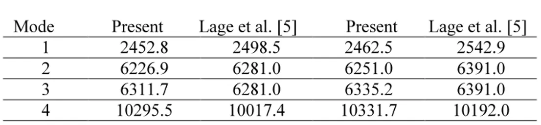
The simple supported square plate of case II is analysed. The side is equal L=1 m but now the total thickness is H=0.04 m (each lamina with 0.01 m of thickness) and the stacking se-quence is (B/F/F/B). The results obtained using a (6x6) element mesh (72 triangular elements) are shown in Table 1, and compared with those obtained in Lage et al [5]. Elastic plate means that the piezoelectric and magnetic properties are not considered - set to zero. A very good approximation is observed between the results obtained by using the layerwise and single layer models.

elastic plate magneto-electro-elastic plate Mode Present Lage et al. [5] Present Lage et al. [5]

1 2452.8 2498.5 2462.5 2542.9

2 6226.9 6281.0 6251.0 6391.0

3 6311.7 6281.0 6335.2 6391.0

4 10295.5 10017.4 10331.7 10192.0

Table 1. Natural Frequencies (rad/s): L=1 m ; H=0.04 m for B/F/F/B plate

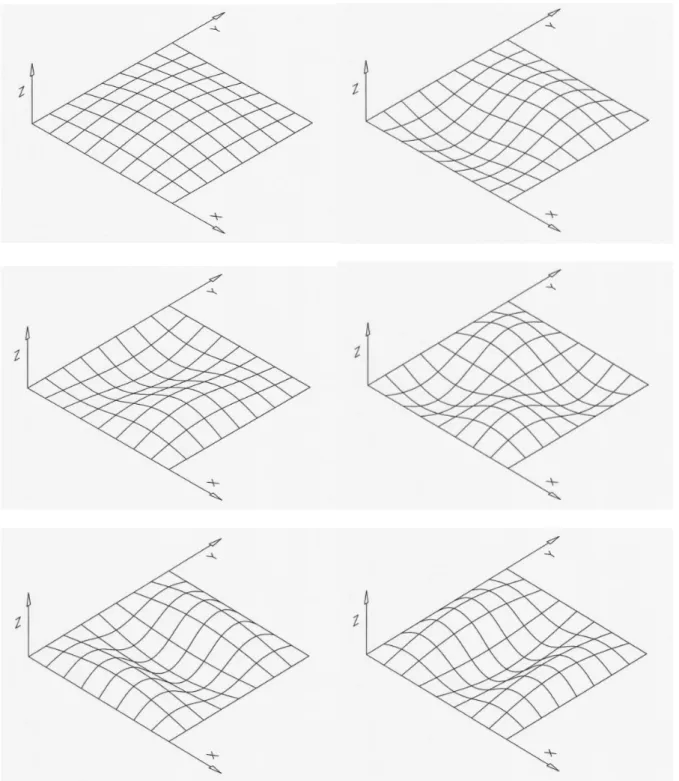
Secondly the plate of case I with different stacking sequences is analysed. The results ob-tained are given in Table 2. In Fig 8 are shown the first six mode shapes of (F/B/F) plate stacking sequence.

elastic plate magneto-electro-elastic plate Mode B only F only B/F/B F/B/F B only F only B/F/B F/B/F

1 12600.01 14882.24 12751.45 14738.18 12631.77 14905.91 12783.17 14761.57 2 24926.81 27965.02 25211.44 27664.41 24964.69 27987.31 25249.50 27686.12 3 25147.20 28198.62 25433.88 27895.27 25185.42 28221.14 25472.28 27917.20 4 34176.64 37478.54 34566.57 37048.92 34210.58 37496.29 34601.21 37065.91 5 39204.94 42568.46 39657.88 42059.00 39234.02 42582.32 39687.79 42072.00 6 39963.98 43475.44 40422.48 42960.06 39995.27 43490.76 40454.58 42974.49

Table 2. Natural Frequencies (rad/s) : L=1 m ; H=0.3 m – HSDT 6 CONCLUSIONS

In this paper a finite element model based on a higher-order plate theory is developed for the static and free vibration analyses of magneto-electro-elastic plates. This model allows to obtain in static analysis the through-thickness distributions of primary variables- mechanical displacements, electric potentials and magnetic potentials-as well as for electric displacements and magnetic inductions. Some results were compared with those obtained by Lage et al. [4] that use a partial mixed layerwise finite element model, and good agreement is found. It should be observed that the layerwise theory allows to the cross-thickness variation of the transversal displacement w, and the corresponding strainε_zz, which is relevant in the stresses results, but essentially in the electric and magnetic potentials as well in electric displacement and magnetic induction. In the free vibration analysis, the results obtained by using the two different models, shown in Table 1, are of the same magnitude, but the quite difference

be-tween the layerwise approach and the single layer formulation of the present model, justifies the discrepancies found between the results.

Figure 8. The first six mode shapes of F/B/F plate ACKNOWLEDGMENTS

The authors thank the financial support of POCTI/FEDER, POCI(2010)/FEDER, Funda-ção para a Ciência e Tecnologia (FCT), POCI/EME/56316/2004, and EU through FP6-STREP project contract Nº 013517- NMP3-CT-2005-0135717.

REFERENCES

[1] E. Pan, Exact solution for simply supported and multilayered magneto-electro-elastic plates. Journal of Applied Mechanics, 68, 608-618, 2001.

[2] E. Pan and P.R. Heyliger, Free vibration of simply supported and multilayered mag-neto-electro-elastic plates. Journal of Sound and Vibration, 252(3), 429–442, 2002. [3] J. Wang, L. Chen, and S. Fang, State vector approach to analysis of multilayered

mag-neto-electro-elastic plates. Inter. Journal of Solids and Structures, 40, 1669-1680, 2003. [4] R.M. Garcia Lage, C.M. Mota Soares and C.A. Mota Soares, Layerwise partial mixed

finite element analysis of magneto-electro-elastic plates. Computers and Structures, 82, 1293-1301, 2004.

[5] R.M. Garcia Lage, C.M. Mota Soares and C.A. Mota Soares, Static and free vibration analysis of magneto-electro-elastic laminated plates by a layerwise partial mixed finite element model. The 3rd

Internacional Conference on Structural Stability and Dynamics, Kissimmee, Florida, USA, 2005.

[6] W.Q. Chen, K.Y. Lee and H.J. Ding, On free vibration of no-homogeneous transversely isotropic magneto-electro-elastic plates. Journal of Sound and Vibration, 279, 237-251, 2005.

[7] F. Ramirez, P.R. Heyliger and E. Pan, Free vibration response of two-dimensional mag-neto-electro-elastic plates. Journal of Sound and Vibration.

http://dx.doi.org/10.1016/j.jsv.2005.08.004.

[8] J.N. Reddy, Mechanics of laminated composite plates and Shells. Boca Raton: CRC Press, 2nd ed., 2004.

[9] O.C. Zienckiewicz, The finite element method in engineering sciences. London: McGraw-Hill, 3rd ed., 1977.