SRef-ID: 1432-0576/ag/2004-22-901 © European Geosciences Union 2004
Annales
Geophysicae
Auroral E-region electron density height profile modification by
electric field driven vertical plasma transport: some evidence in
EISCAT CP-1 data statistics
T. B¨osinger1, G. C. Hussey2, C. Haldoupis3, and K. Schlegel4
1Department of Physical Sciences, University of Oulu, Oulu, Finland
1Institute of Space and Atmospheric Studies, University of Saskatchewan, Saskatoon, Canada 3Physics Department, University of Crete, Iraklion, Crete, Greece
4Max-Planck-Institut f¨ur Aeronomie, Katlenburg-Lindau, Germany
Received: 27 September 2002 – Revised: 31 July 2003 – Accepted: 12 August 2003 – Published: 19 March 2004
Abstract.A model developed several years ago by
Huusko-nen et al. (1984) predicted that vertical transport of ions in the nocturnal auroral E-region ionosphere can shift the elec-tron density profiles in altitude during times of sufficiently large electric fields. If the vertical plasma transport effect was to operate over a sufficiently long enough time, then the real height of the E-region electron maximum should be shifted some km upwards (downwards) in the eastward (westward) auroral electrojet, respectively, when the elec-tric field is strong, exceeding, say, 50 mV/m. Motivated by these predictions and the lack of any experimental ver-ification so far, we made use of the large database of the European Incoherent Scatter (EISCAT) radar to investigate if the anticipated vertical plasma transport is at work in the auroral E-region ionosphere and thus to test the Huuskonen et al. (1984) model. For this purpose a new type of EIS-CAT data display was developed which enabled us to order a large number of electron density height profiles, collected over 16 years of EISCAT operation, according to the electric field magnitude and direction as measured at the same time at the radar’s magnetic field line in the F-region. Our anal-ysis shows some signatures in tune with a vertical plasma transport in the auroral E-region of the type predicted by the Huuskonen et al. model. The evidence brought forward is, however, not unambiguous and requires more rigorous anal-ysis.
Key words. Ionosphere (auroral ionosphere; plasma
con-vection; electric fields and currents)
1 Introduction
Since 1984, European Incoherent Scatter radar, EISCAT, has been producing in regular intervals, through its Common Program (CP) experiments, measurements of basic plasma parameters of the auroral ionosphere. A large and still
grow-Correspondence to:T. B¨osinger ([email protected])
ing database is now available, which allows not only for anal-ysis of long-term trends over many years, but also for investi-gation into effects which are buried under the dominant pro-cesses. In this work, some 12 000 E-region electron density profiles were used in conjunction with concurrent F-region electric field measurements to look for experimental verifi-cation of what is called in the following the VPT (vertical plasma transport) effect. With the electric fieldE and the ambient magnetic fieldBthe plasma convectionE×B im-plies a vertical component,vzifBis inclined with respect to the vertical. This inclination effect is principally the same in the E as well as the F-region, but the phenomenon has in the E-region less of a chance to leave a measurable signature.
As is well known VPT plays a crucial role in the physics and chemistry of the F-region. On the other hand, there is some speculation that VPT effects might also be of impor-tance in the E-region under conditions of low electron den-sity and large electric fields. This was suggested by Huusko-nen et al. (1984) in a theoretical analysis on how the electric field induced vertical plasma convection could influence the precipitation E-layer in the auroral ionosphere. According to their model, a distinct re-shaping of the electron density height profile is to be expected in the presence of a suffi-ciently large E-field. If this effect exists, it will have sub-sequent consequences on all derived ionospheric parameters and also on the excitation of E-region plasma instabilities (e.g. see Haldoupis et al., 2000).
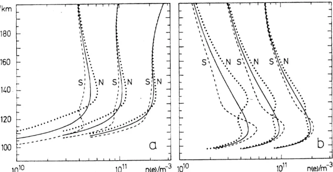
Fig. 1.Each panel shows auroral electron density profiles generated by precipitating electrons of three different flux densities. The continuous curves are valid in the absence of an electric field and the dotted and dashed ones correspond to a field of 50 mV/m directed towards magnetic
north and south, respectively. The characteristic energy of the incident electron spectrum is 1 keV in panel(a)and 3 keV in panel(b)(from
Huuskonen et al., 1984; Copyright 1984, with permission).
on experimental verification of the VPT effect on E-region precipitation layers has not yet become available. The dif-ficulties for such an investigation are to be considered even more severe when it is realized that the presumed VPT effect is expected to work along the same direction as the natu-rally occurring particle precipitation patterns, that is, softer particle precipitation in the auroral eastward electrojet (EJ), and harder particle precipitation in the westward electrojet (WJ); see, e.g. the early work by Hartz (1971). As shown by Huuskonen et al. (1984), the northward (southward) E-field, which drives the EJ (WJ), would push the electron density maximum upward (downward) because of VPT, just like the soft (hard) particle precipitation is doing as well.
The paper proceeds as follows: in Sect. 2 the approach by Huuskonen et al. (1984) is briefly reviewed. In Sect. 3 reference is made to EISCAT measurements, and the data archives, and some arguments are given for the choice of data presentation and the type of statistical analysis. In Sect. 4 the statistical trends in the EISCAT database which are of relevance to the present study are visualized in a series of plots so that a decision can be made in favor or against VPT. Finally, since the evidence for VPT effects in EISCAT data turned out to be weak, in Sect. 6 our findings are discussed with the emphasis placed on the possible reasons behind the apparent difficulties in our experimental approach and/or in a deficiency in the mechanism envisaged by Huuskonen et al. (1984).
2 Review of the proposed VPT effects
The starting point of Huuskonen et al. (1984), hereafter re-ferred to as paper H, is that, in addition to the ion production and losses, E-region plasma density can also be affected by vertical ion motions driven by large electric fields. In this scenario, vertical plasma transport is expected to be impor-tant if the distance travelled by an ion before recombination is comparable to, or longer than, the scale length of the elec-tron density profile. At E-region altitudes the lifetimes of di-atomic ions range from about 10 to 100 s for electron densi-ties between 5×10¹¹and 5×10¹⁰m−3, if an effective recom-bination coefficient ofα=2×10⁻¹³m3s−1is used. As shown
by Nygr´en et al. (1984), during periods of strong E-fields in the range from 50 to 100 mV/m, which occur often in the auroral ionosphere during disturbed conditions (e.g. see Opgenoorth et al., 1990 and references therein), the plasma flow can reach maximum vertical speeds between 250 and 500 m/s (see also Fig. 1 in paper H). As discussed in paper H, at these speeds the ions may travel during their lifetimes vertical distances comparable to the thickness of the E-layer; therefore, VPT can lead to significant modifications of the electron density profile. It is important to stress that VPT is a dip-angle effect, since the vertical plasma flow is a conse-quence of a horizontally stratified ionosphere permeated by the Earth’s magnetic field lines which form an oblique angle to the vertical and act as equipotentials.
O molecules (densities given by CIRA-72) were taken to be ionized by precipitating electrons, which leads to the produc-tion of O+2, N+2, O+and N+ions, whereas the NO concen-tration was assumed to be unchanged and given by MacLeod et al. (1975). The semiempirical method of Rees (1963) was used in order to obtain the total ionization rate profile, and the incident electron spectrum was assumed to obey a Maxwellian shape with a given characteristic energy. Also, ion drag and strong heating, as well as neutral wind effects, were neglected. A stationary state was assumed throughout the calculations, which were obtained by solving numerically the ion continuity equation at 75◦magnetic dip, correspond-ing to the field line at the Tromsø EISCAT site. For details, see Huuskonen et al. (1984).
As shown in paper H, the computed electron density pro-files can be altered significantly by VPT effects in the pres-ence of large electric fields. This is illustrated in Fig. 1, which was reproduced from Fig. 2 of paper H for the sake of convenience. Shown there in each panel are computed electron density height profiles for three different flux densi-ties; the solid curves represent the situation when no electric field is present, whereas the rest refer to an electric field of 50 mV/m directed either to the north (N) or south (S). Note that profiles in panels (a) and (b) refer to incident electron en-ergies of 1 keV and 3 keV, respectively. Inspection of Fig. 1 shows that VPT effects on electron density profiles can be clearly identifiable in the auroral E-region, especially during conditions of lower, rather than higher, electron densities.
3 database and processing
In the present analysis a large number of EISCAT CP-1 ob-servations are used. The CP-1 experiment (there are sev-eral versions: F, H, I, J, and K during the years from 1984 to 1998) is the most frequently used configuration, both in the EISCAT Common Programme series (used here through-out) and in the EISCAT Special Programme series. CP-1 is a field-aligned, moderate spatial (3 km) and moderate tem-poral (2 min; in early versions 5 min) resolution experiment. It covers for the high range resolution modes (multi-pulse before version J, alternating code for J and K) the height from about 90 to 240 km (CP-1-F had a maximum height of
∼170 km), and is scheduled to run regularly for 24 or more continuous hours. The radar antenna at Tromsø, Norway is oriented to observe along the direction of the local magnetic field line. In addition, remote receiver radars at Kiruna, Swe-den (KIR) and Sodankyl¨a, Finland (SOD), along with the Tromsø (TRO) radar, measure the plasma drift velocity in the F-region at an altitude of∼280 km. At this altitude the plasma driftsE×vecBand, as such, the electric field can be easily calculated and assumed to map down to the E-region.
Although CP-1 has undergone various modifications and improvements (e.g. the multi-pulse data was replaced by an alternating code scheme in versions J and K), since its imple-mentation in 1984 this experiment has regularly provided E-and F-region parameters, such as electron density E-and
tem--90 0 90 180 270
E-field azimuth (deg E of N) 0
20 40 60 80 100
E-field magnitude (mV/m)
EISCAT CP1 Occurrence Distribution
night hours; number of profiles: 9771 (ne)peak < 10 x 1011 m-3; |E| > 0 mV/m
0 10 20 30 40
-90 0 90 180 270
0 20 40 60 80 100
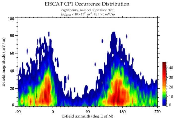
Fig. 2.The occurrence distribution plot of the electric field magni-tude versus its azimuth for the night hours, which have been defined as those between 17:00 and 07:00 MLT (16:00 to 06:00 UT). East-ward electrojet (EJ) conditions correspond to a northEast-ward directed
E-field (azimuth∼0◦), while westward electrojet (WJ) conditions
correspond to a southward directed E-field (azimuth∼180◦). The
bin size for E-field magnitude is 5 mV/m, and for E-field directions 3◦.
perature, ion drift velocity and temperature, and electric field measurements, since that time. The electron densities used in our analysis are corrected to account for unequal tempera-tures and Debye-length effects (e.g., see Schlegel, 1988) and are regularly calibrated with the help of ionosonde data. In general, the uncertainties in the incoherent scatter measure-ments are expected to be in the range of 5 to 10%, depend-ing on the signal-to-noise ratio (SNR). In the analysis only those profiles are considered for which the SNR was reason-ably high (SNR≥0.02). This threshold has also been applied to the electric field measurements: SNR(SOD) had to be
≥0.02; SNR(TRO) and SNR(KIR) are generally higher. The database of CP-1 measurements for this study was obtained from the CP-1 data archived at the Max-Planck-Institut f¨ur Aeromonie in Lindau, Germany.
For every valid E-region profile in the EISCAT data set, besides the electric field (both magnitude and azimuth) mea-surements, the “mean” electron density (ne)peak, and the “mean” height or altitudeh{(ne)peak}, or simply hpeak, of the electron density peak or maximum, were calculated and stored. Then different combinations of these parameters were plotted against one another as self-normalized occur-rence distributions (2 dimensional histograms), i.e. data are binned and counted with respect to how often they are ob-served.
-90 0 90 180 270 E-field azimuth (deg E of N)
EISCAT CP1 Occurrence Distribution
night hours; number of profiles: 9765 (ne)peak < 10 x 1011 m-3; |E| > 0 mV/m
0 10 20 30 40 50
-90 0 90 180 270
90 100 110 120 130 140 150
Altitude at n
e
peak (km)
Fig. 3.The occurrence distribution plot of the altitude of the
elec-tron density peakhpeak(i.e. the altitude at thenepeak or maximum,
h{(ne)peak}) as a function of the E-field azimuth for the night hours.
The bin size for altitude is 3 km, and for E-field directions 3◦.
keep in mind since the number of occurrence is a different property of the physical quantity than the quantity itself. The width of a distribution should not be mixed with the width of the quantity (whatever it is, e.g. electron density maximum). The electric field vector is calculated fromV=E×B/B2, whereBis the geomagnetic field along the EISCAT viewing direction (assumed fixed) andV is the plasma drift velocity vector at an altitude of∼280 km computed from the mean Doppler shifts at the three EISCAT receivers (TRO, KIR, and SOD). The electric field vector is defined using a right-handed coordinate system (north, east, down). From this, the horizontal E-field magnitude, |E|, given in units of mV/m, and the (horizontal) E-field azimuth, given in degrees east of north, are calculated from the north and east components of the electric field vectorE.
In order to define more accurately the electron density peak and the height at which it occurs, “mean” values were determined. The “mean” electron density at the electron den-sity peak(ne)peak was calculated by averaging the electron densities, ±2 height bins about the peak electron density height bin. That is,
(ne)peak= +2
X
i=−2
ne(p+i)
5 , (1)
where ne(p+i)is the electron density at height or altitude binp+i andp is the height bin of the peak or maximum electron density.
Similarly, the “mean” height hpeak=h{(ne)peak} at the electron density peak is calculated by performing a height average, which is weighted by the corresponding electron density,±2 height bins about the peak electron density height
bin. That is,
hpeak =h{(ne)peak} = +2
X
i=−2
h(p+i)∗ne(p+i)
+2
X
i=−2
ne(p+i)
, (2)
wherene(p+i), andphave the same meaning as above and
h(p+i) is the actual height in km at height binp+i. Al-though the search for the electron density maximum was car-ried out up to a maximum altitude of 180 km, in our analysis plots were created only to an altitude of 150 km.
4 EISCAT statistics in search for VPT
During the EISCAT operation, the magnetic field line tan-gential to the radar’s field of view covers a certain range of L-values (L=6.0 to 12) in all local time sectors due to vary-ing magnetic activity accordvary-ing to Tsyganenko’s TS89 model Tsyganenko (1989). This coverage of L-values is also the case for low altitude polar orbiting satellites, such as those from the DMSP and NOAA programmes. From the prop-erties of precipitating particles detected by these satellites, electron density height profiles have been derived on a rou-tine basis, providing data suitable for large statistical studies “(e.g. Hardy et al., 1985, 1987; Newell et al., 1996).” Since each observational platform has its own advantages and dis-advantages (e.g. the L-value range of EISCAT measurements is rather limited), one may ask for the specific merit of EIS-CAT observations in the given context, which, without a doubt, is the electric field measurements. Surveys of parti-cle precipitation patterns obtained from low altitude satellites cannot be easily ordered according to electric field proper-ties. Another strong merit of EISCAT is its long-term obser-vations, although one may argue that some of the mentioned satellite programmes also have long-term observations.
-90 0 90 180 270 E-field azimuth (deg E of N)
EISCAT CP1 Occurrence Distribution
night hours; number of profiles: 9781 (ne)peak < 10 x 1011 m-3; |E| > 0 mV/m
0 5 10 15 20 25 30 35
-90 0 90 180 270
0 2 4 6 8
ne
at altitude peak (10
11 m -3)
Fig. 4.The occurrence distribution plot of the electron density peak
(ne)peak as a function of the E-field azimuth for the night hours.
The bin size for electron density is 0.2·1011m−3, the one of E-field
directions 3◦.
(∼5 mV/m); and 4) large electric fields are either northward or southward (at least at the EISCAT latitude). Therefore, judging from the electric field properties alone, E-region electron density height profile modification by large electric field driven VPT can be expected equally well during EJ and WJ conditions. This suggests a high preference for a VPT ef-fect to occur in the local time sectors centered around 01:00 and 16:00 MLT (00:00 and 15:00 UT).
In Fig. 3, the occurrence frequency of the altitude of the electron density maximum(ne)peak, hereafter referred to as
hpeak, is displayed as a function of the E-field azimuth, again for the night hours. Two features are clearly noticed: 1) the most probablehpeak in the EJ is∼120 km, which is about 12 km higher than the most probable height in the WJ where it is∼108 km; and 2) moreover, thehpeakis less well defined with respect to altitude (height) in the EJ (width of height distribution is ∼20 km) than in the WJ (width ∼10 km), while the opposite is the case with respect to E-field azimuth, wherehpeakin the EJ is confined to a smaller range of E-field azimuths (width of angle distribution∼20◦) than in the WJ (width∼50◦).
It is a well-known fact, confirmed by many statistical sur-veys on particle precipitation properties obtained from low altitude polar orbiting satellites (e.g. Hardy et al., 1985), that the difference between thehpeak in the EJ as compared to the WJ, is due to the difference in the hardness of the pre-cipitating particles. This also shows up in the mean altitude of the electrojets (Kamide and Brekke, 1977; Sugino et al., 2002). If we take the values ofhpeak given above (Fig. 3), and assume for the sake of simplicity solely electron precipi-tation, the difference in the characteristic energies, assuming isotropic pitch angle and Maxwellian energy distributions, is of the order of 2 keV in the EJ versus 5±2 keV in the WJ (Auroral Physics Program for Science and Education). This is compatible with values given in the literature for electron precipitation (Hardy et al., 1985), though a bit high for the
0 20 40 60 80 100
E-field magnitude (mV/m)
EISCAT CP1 Occurrence Distribution
Eastjet; night hours; number of profiles: 4203 (ne)peak < 10 x 1011 m-3; |E| > 0 mV/m
0 20 40 60 80 100
0 20 40 60 80 100
90 100 110 120 130 140 150
Altitude at n
e
peak (km)
0 20 40 60 80 100
E-field magnitude (mV/m)
EISCAT CP1 Occurrence Distribution
Westjet; night hours; number of profiles: 5539 (ne)peak < 10 x 1011 m-3; |E| > 0 mV/m
0 50 100 150
0 20 40 60 80 100
90 100 110 120 130 140 150
Altitude at n
e
peak (km)
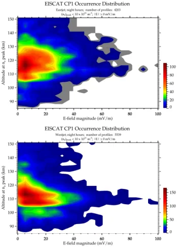
Fig. 5. The occurrence distribution plot of the altitude of the
elec-tron density peakhpeakas a function of the E-field magnitude|E|
for the night hours during eastward electrojet conditions (top) and the one for westward electrojet conditions (bottom). The bin size
for altitude is 3 km, and for E-field directions 3◦.
characteristic energy in the EJ. Two things should, nonethe-less, be realized: (1) the EISCAT electron density profile does not differentiate between an E-region precipitation and a photoionization peak, (2) our definition of day and night hours is ordering the data primarily into two LT sectors; re-call that at times the ionosphere is sunlit or dark for 24 h of the day.
0 20 40 60 80 100 E-field magnitude (mV/m)
EISCAT CP1 Occurrence Distribution
Eastjet; dark hours; number of profiles: 1152 (ne)peak > 0.0 x 10¹¹ m-3; |E| > 0 mV/m
0 5 10 15 20 25
0 20 40 60 80 100
90 100 110 120 130 140 150
Altitude at n
e
peak (km)
0 20 40 60 80 100
E-field magnitude (mV/m)
EISCAT CP1 Occurrence Distribution
Eastjet; sunlit hours; number of profiles: 2550 (ne)peak > 0.0 x 10¹¹ m-3; |E| > 0 mV/m
0 10 20 30 40
0 20 40 60 80 100
90 100 110 120 130 140 150
Altitude at n
e
peak (km)
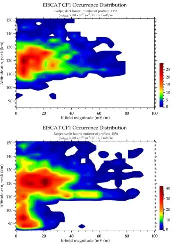
Fig. 6.The same as Fig. 5 (top) but for a dark ionosphere (top) and a sunlit ionosphere (bottom).
VPT effects should be more effective in regions and pe-riods of low electron density. The chances of meeting the low electron density criterion is definitely higher for EJ (dif-fuse auroras) than for WJ (substorms) conditions. This is evident in Fig. 4, which shows the occurrence distribution of the electron density profile maximum(ne)peakas a function of E-field azimuth. As is seen,(ne)peak values are smaller and more confined in azimuth in the EJ than they are in the WJ.
A closer look at EJ conditions alone in Fig. 5 (top), where the occurrence distribution ofhpeakversus E-field magnitude is plotted, reveals the following. The height distribution of
hpeak is centered at ∼117 km for low electric field values and tends to become bifurcated around 30 mV/m (113 and 123 km), and for large electric fields (|E|≥40 mV/m) tends to level off at 112 km. The bifurcation could be associated with different mechanisms, and the slight trend to go up and down in altitude for moderate fields in particular, to the VPT effect. We will discuss these findings in greater detail below and proceed to the counter example, the WJ situation, as pre-sented in Fig. 5 (bottom). Here a VPT effect should act in the downward direction. As can be seen, the height distribution ofhpeak in the WJ exhibits a tendency of decreasing height with increasing|E|, again for moderate electric fields (0 to
40 mV/m) and tends to level off at an altitude of∼112 km for large electric field values (|E|≥40 mV/m).
Figure 5 should be seen vis-`a-vis Fig. 4 of paper H. One cannot but admit that the overall impression in the ing features of Fig. 5 exhibits some similarity in the contrast-ing features (liftcontrast-ing and lowercontrast-ing ofhpeak with|E|) seen in Fig. 4 of paper H. The shifts are not on scale but qualitatively they are there and in the right direction.
It is interesting that for large E-field values the height of
hpeak seems to level off at the same altitude in the WJ, as well as in the EJ, at about 112 km (cf. Fig. 5). This property is a persistent feature of all ourhpeakdistribution versus|E|, regardless of LT and solar illumination (dark or sunlit). It will be discussed in greater detail below.
Let’s now have a closer look to the situation in the EJ but choosing specifically the situation of a dark ionosphere and the one of a sunlit ionosphere (due to the high latitude, the ionosphere, at an altitude of 100 km above the EISCAT radar, is sunlit for 24 h from about 13 April to 26 August and dark for almost 24 h from 24 November until 31 January) In Fig. 6 the occurrence frequencies ofhpeakare displayed for purely dark (top) and purely sunlit (bottom) ionospheric conditions. Figure 6 contains new details:
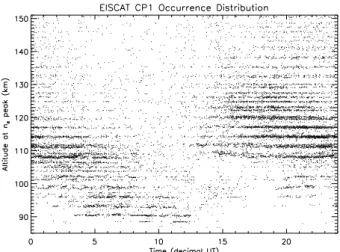
Regarding the EJ of the sunlit ionosphere, Fig. 6 (bottom), the first to be noticed is ahpeak at 93 km. We associate it with energetic particle precipitation and partially with pho-toionization of the D-region. The main contribution to this peak comes from the local morning time sector which can be easily verified from Fig. 7 (note that there is a high latitude EJ in the morning sector). This peak has no “access” to VPT, since vertical ion transport is limited to heights above 100 km under any E-field direction (cf. Fig. 1 in paper H). Moreover, the 05:00 to 10:00 UT local time sector is characterized by small electric field values because of the large ionospheric conductances (figure with electron density not shown).
The second to be noticed in Fig. 6 (bottom) is the – al-ready earlier focused – levelling-off ofhpeak at an altitude close to 112 km, from medium to large electric fields. It is a pronounced signature in contrasting evidence to the situation of the dark ionosphere (Fig. 6, top).
Thehpeak at 110/113 km in Fig. 6 (bottom and top) for vanishing E-fields we associate primarily with photoioniza-tion which could be easily verified by running the Interna-tional Standard Ionosphere (IRI) model for the EISCAT site coordinates, and LT sectors of the EJ for various solar activ-ity levels.
Regarding the EJ of the dark ionosphere, Fig. 6 (top), the first to be noticed is that the levelling-off ofhpeak at around 112 km is less distinct and disappears practically for very large E-fields. Second, there is clear evidence for an ascend-ing hpeak with increasing E-field magnitude, starting from
∼120 km, reaching∼125 km for 20 mV/m, and 130 km for 40 mV/m. The trend continues up to 60 mV/m, with poor statistics, however.
more pronounced than in Fig. 5 (top). Figure 6 (top and bottom) shows an assent and descent of a peak, starting from∼30 mV/m E-field values, and consequently, a widen-ing/deepening of the bifurcation. Such a behavior is con-sistent with a VPT effect acting on a low density hpeak in a proper height range. Why does this effect not show up as clearly in Fig. 5 (top)? Well, actually it is also present in Fig. 5 but a superposition of photoionization and particle pre-cipitation may result in a smearing out of preferential peaks. There is a greater plasma supply from low altitudes in the sunlit ionosphere (cf. Fig. 6, bottom).
5 Discussion
The experimental findings presented above can be summa-rized as follows: we were able to pinpoint signatures in the
hpeak height distribution as a function of|E|, which can be interpreted in terms of a VPT effect. We focused finally on the EJ and could show there is an ascend ofhpeak with in-creasing E-field strength, as predicted by theory, and a grow-ing/deepening bifurcation in thehpeak distribution, starting around 20 to 30 mV/m. These signatures are more pro-nounced in the dark as compared to the sunlit ionosphere, but they are present in both. Also, the WJ exhibit a decline ofhpeak, accompanied by an increase in|E|. All these sig-natures are compatible with VPT. Our experimental findings in favor of VPT are, however, not unambiguous. A verifica-tion of VPT requires large electric fields, preferentially ex-tremely large fields, as the best test case. Those fields are unfortunately rare. Our statistics can be regarded as being still good in the intermediate E-field range, let’s say from 30 to 60 mV/m.
One may ask: is the statistical approach at all appropriate for the type of questioning? In general, a random distribu-tion around a mean value will average to zero when taking the overall average; a systematic shift to either side of the mean will, however, not average out. If VPT is to exist, it will produce a systematic shift on either side of the zero E-field peak. Moreover, we have effective tools to sort the data by all relevant parameters. It allows one to study the sta-tistical properties of the relevant quantities as such (E-field magnitude and its direction, the E-region peak height and its electron density values). Thereafter, we can distinguish between local time sectors (dayside and nightside) and be-tween, either precipitation layers alone, or a combination of precipitation and photoionization layers (dark versus sunlit ionosphere). This helps us to find the optimal conditions for revealing VPT effects, if they exist.
We interpret Fig. 6 (top) as follows. The peak at 120 km is submit to VPT, resulting in an upward shift towards 130 km at around 60 mV/m. The peak at 113 km is not very much affected by VPT and gains only some km in height, if any. Moreover a secondary peak is produced from the upshifted one which is a consequence of an erosion of the primary peak at 120 km. This secondary peak is asymptotically approach-ing the peak at 112 km. The bifurcation is widenapproach-ing with
in-Fig. 7. A scatter-plot of hpeak as a function of local time
(LT=UT+1.25 h). Each point indicates the altitude of the electron density maximum of an individual height profile.
creasing E-field, starting from some 20 to 30 mV/m onwards (Figs. 5 and 6).
Since our algorithm identifies only the main maximum in the electron density height profile, the question arises of how can we address/discuss a “secondary” peak. Even a quick survey of the EISCAT CP1 density height profiles could show that the data is usually too noisy to identify fine struc-tures in the profile. Under these conditions it is of utmost concern to look for an absolute maximum, especially when using an automatic algorithm. A brief exercise can further demonstrate: when adding random noise of discriminating amplitude to an analytic double peak structure and determin-ing the absolute maximum, statistically it will yield an oc-currence frequency with a maximum at the higher twin peak and a second maximum at the lower twin peak. Thanks to noise, a double peak structure is statistically resolvable even by looking for an absolute maximum alone.
A double peak structure, however, is not necessarily proof of VPT. A twin or even multi-peak structure may reflect the inhomogeneity of our data. It may also be a consequence of two different ionization processes (particle precipitation and photoionization), each of it operating with largest efficiency in a different height range. Also, VPT acts differently de-pending on the height of maximum ion production relative to the height of maximal operative VPT (for northward E-field there is a maximum vertical ion speed at 120–125 km, which drops down by close to one order of magnitude to 10 km on either side of this height (cf. paper H, their Fig. 1). Therefore, VPT is not necessarily associated with a growing/depending bifurcation when the E-field increases. If the maximum pro-duction height coincides with the height of maximum VPT efficiency, an enhanced northward E-field would not produce a secondary peak, but instead increase the primary peak’s electron density by thinning it (cf. paper H, their Fig. 3a).
with the EJ or WJ (cf. Fig. 5), is an important experimental finding. The following options exist for an interpretation:
Interpretation A: it is due to photoionization which is in-dependent of the E-field in direction and strength and can, therefore, easily provide an explanation as to why it is en-countered in the EJ as well as the WJ. A quick run of the IRI model for the EISCAT electron density height profile can fur-ther tell that photoionization controls the electron density at E-region heights to a considerable extent.
Interpretation B: thehpeaktends to level off at a height of
∼112 km because(ne)peakis so high that VPT cannot affect the peak height even in the case of very large electric fields. Therefore it is independent of|E|and levels off at the most probable peak altitude.
Interpretation C: levelling-off ofhpeak at∼112 km is to be seen in the context of anomalous heating due to Farley-Buneman instability in association with Hall currents which flow preferentially at this altitude (Schlegel and St.-Maurice, 1981; Wickwar et al., 1981). The fact that this feature ap-pears in our statistics shows the high occurrence of this in-stability (cf. Hussy et al., 2002).
Interpretation D: it is a by-product of VPT.
To interpretation A: it can be checked by comparing the dark ionosphere of Fig. 6 (top) versus the sunlit ionosphere of Fig. 6 (bottom). Thehpeak around 112 km is much less pronounced in the dark as compared to the sunlit ionosphere, although it has not entirely disappeared. Note that above EISCAT, at an altitude of 100 km, the ionosphere is even on 21 December, at local noon, not entirely dark (the Sun is only 3.5◦ below horizon). A further check (not shown) by choosing a really dark ionosphere, at the local time sector 16:00 to 17:00 UT, told us that for large electric fields,hpeak still tends to level off at a height of∼112 km. Thus, it cannot be due to photoionization (cf. Figs. 5 and 6). Interpretation A is wrong.
To interpretation B: can be excluded right away. Large, especially, very large electric fields are not encountered when the electron density is high. We ordered our statistics also according to(ne)peak(not shown). The peak at∼112 km is a persistent signature in all ourhpeak distributions even for
(ne)peak<1011m−3. Interpretation B is also wrong.
To interpretation C: the context might be right but it is not clear how a small-scale instability such as Farley-Buneman can largely affect the electron density. The increase in elec-tron temperature and associated decrease in the recombi-nation coefficient and resulting increase in electron density should modify the electron density by some percent only. In-terpretation C is not sufficient.
To interpretation D: As outlined above VPT may generate a double peak structure (cf. Fig. 1). A secondary maximum may be generated. In the EJ (WJ) the primary peak is pushed up (down), whereas the secondary peak is going down (up). In all ourhpeakheight distributions (cf. Figs. 5 and 6) signa-tures of a bifurcation are encountered. In addition, the bifur-cation is widening/deepening with increasing E-field. Inter-pretation D is at least compatible with VPT, however, accord-ing to the modellaccord-ing in paper H – the down-shifted peak in
the EJ is always smaller than the upward shifted. It remains a mystery why in Fig. 6 (bottom) the levelling-off peak at 113 km exhibits the highest occurrence frequency. It may be due to the coincidence of two peaks, a down-shifted sec-ondary peak with a photoionization peak of constant height (cf. Fig. 6; bottom).
In an earlier stage of our investigation we believed that the height of maximum ion production due to (soft) particle precipitation is in the EJ not getting down enough in the E-region to make a noticeable VPT effect. As Figs. 5 (top) and 6 (top) can tell us, thehpeak distribution includes the height range from 110 to 130 km and covers nicely the most effec-tive height range for VPT (125 km). It may look surprising that in the EJ an electron density peak is frequently encoun-tered at an altitude so low as 112 km (cf. Fig. 6; top). In the 15:00 to 19:00 UT time sector the ionospheric trough is fre-quently intersected by the EISCAT magnetic field line. In the trough region the electron density height profile at the EIS-CAT field line is determined mainly by proton precipitation which produces, according to Hardy et al. (1991) an electron density maximum at∼120 km for Kp=3, the best represented Kp value in our data. This may be the reason for the “pre-existing” twin peak of the dark (only precipitation affected) ionosphere.
Summarizing, it can be said: EISCAT CP-1 data statistics provides some evidence for the existence of a VPT effect. In spite of considerable efforts, we were, however, not able to demonstrate the existence of VPT beyond any doubt. Other methods and/or data have to be developed/found for the final answer.
Some problems inherent to the EISCAT radar measure-ment should be here measure-mentioned: the CP-1 data altitude reso-lution of 3 km is, in fact, not enough to infer shifts ofhpeak which are of the same order. An upward shift from 120 to something like 135 km, as encountered in Fig. 6 (top), in-volves in any case more than 2 discrete steps (cf. Fig. 7) and allows access tohpeakvalues even in between.
We finish by addressing some critical points of the VPT theory itself; some of them were already mentioned by Hu-uskonen et al. (1984). The authors of paper H estimated the lifetime of the ions assuming a value of the effective recom-bination coefficient ofα=2×10⁻¹³m3s−1. In 1992, Nygr´en
et al. (1992) published a report on a novel EISCAT measure-ment ofα, using the decay of the electron density after peri-ods of short-lived (∼4 s) auroral precipitation bursts. Their measurement (for a review on earlier works, see Nygr´en et al., 1992 and references therein) was at this time the most precise measurement in the height range from 85 to 115 km. Re-analysis of the same data by Ulich et al. 2000 yielded an even higher precision by allowing a time dependentαduring the precipitation events and the process of electron density decay. This approach was made possible by the use of the Sodankyl¨a Ion Chemistry model of Turunen et al. (1996). Now, if we use this most recent value ofα=4×10⁻¹³m3s−1
in turn, means that the lifetimes of the ions estimated in paper H now could “decrease” by a factor of two, yielding 5 to 50 s (instead of 10 to 100 s) for the ion lifetimes calculated using their assumed electron densities. The effective recombina-tion coefficient is a funcrecombina-tion of height and temperature. The authors in paper H were certainly not wrong in their order of magnitude estimate, but a more realistic value ofαtells us that the chances for a VPT effect to be detected are smaller than paper H suggests.
In the modelling of paper H a static neutral atmosphere is assumed, particularly a constant NO concentration taken from MacLeod et al. (1975). Recent model calculations based on an updated version of the Sodankyl¨a Ion Chem-istry model (Turunen et al., 1996) also including now neutral chemistry ( Ulich et al., 2001), showed that the NO concen-tration is accumulating by a persistent electron precipitation. However, since NO is a minor constituent of the E-region neutrals and the major constituent NO+ within the E-region ions is not formed from the neutral NO population (Rees, 1989) we believe that in paper H the assumption of a constant NO concentration (although not realistic) is not signaling a major defect of the model. This also holds for neglecting ion collisions with NO neutrals. Unfortunately the Sodankyl¨a Ion Chemistry model does not yet include vertical transport, otherwise its use would have been the most straightforward approach to check the validity of the ionosphere model in paper H.
More severe is that in paper H, ion drag, strong heating, as well as neutral wind effects, were neglected. Heating elec-trons lead for any given production rate to an increase in electron density through a reduction in the recombination rate (Schlegel et al., 1982; St.-Maurice et al., 1999). To our knowledge there is no report on long-term averages of neutral wind behavior. We did an exercise on this topic by computing the annual means of neutral wind induced ver-tical ion velocity in E-region heights as a function of local time using a numerical model (Voiculesu; private communi-cation). At 120 km, in the afternoon sector (EJ), the annual mean is downward and can, in fact, reach considerable am-plitudes (70 m/s). This may contribute to the levelling-off of
hpeak at 112 km. Above all, it is, however, to be noted that ion drag/wind effects operate on the order of hours (say, at least 3 h to have any noticeable effect; see, e.g. Johnson et al., 1987) and seeing that VPT is to operate on the order of minutes, then one would assume that drag/wind effects can be ignored. Ion drag and neutral wind effects are not a persis-tent signature of the peak E-region ionosphere. In a statistical sense, therefore, it seems justified to neglect those effects.
In summary, the most critical points of E-region VPT are to be seen: first, the lifetime of ions is short and may be even shorter than that which the authors of paper H assumed (see above). Second, only a zonal electric field produces a VPT bulk motion up or downward of the entire height region including E- and F-regions (paper H, their Fig. 1). The ionospheric E-field is, however, basically a meridional field and the zonal E-field remains small (cf. Fig. 2). Large meridional E-fields produce a noticeable VPT effect only in
a narrow height range (see above). Finally, there are – to our knowledge – no quantitative estimates available whether or how much, neutral wind induced vertical ion velocities change the scenario of VPT.
The emphasis of our study lies on the usage of CP-1 data. We are asking what can we learn from its statistics in view of VPT. It is not within the scope of this paper to go through other possible scenarios of VPT verification. It became obvi-ous in the course of our study that it is difficult to demonstrate a VPT effect beyond any doubt but we forwarded – to our mind – rather intriguing signatures in favor of the existence of VPT which should provide enough motivation for a more rigorous analysis. Everything that we are discussing here could be, in fact, modelled, including realistic geophysical conditions with electron and proton precipitation and pho-toionization. Also, a more realistic up-to-date ionospheric E-region model is necessary, that is capable of providing non-steady-state solutions for vertical plasma transport under time varying conditions of E-region plasma recombination.
The study of the VPT effect is not only of academic inter-est. Even if VPT proves to be a very minor effect, it may have further reaching consequences in the context of E-region in-stabilities (e.g. see Haldoupis et al., 2000). A thinning or fat-tening and/or upward/downward shift of the electron density maximum has a magnifying effect on the vertical gradient of the electron density height profile and its “operating” altitude for e.g. the Farley-Buneman instability.
Acknowledgements. We are indebted to the director and staff of EISCAT for operating the facility and greatly acknowledge the sup-port of all the individuals and personnel of this institution. The EIS-CAT Scientific Association is supported by Suomen Akatemia (Fin-land), the Centre National de la R´echerche Scientifique (France), the Max-Planck Gesellschaft (Germany), the Science and Engineer-ing Research Council (UK), Norges Almenraitenskapelige Forskn-ingsr˚ad. (Norway), Naturvetenskapliga Forskningsr˚adet (Sweden), and the National Institute of Polar Research (Japan). Support for G.C.H. for this research by the National Science and Engineering Research Council (NSERC) of Canada is also gratefully acknowl-edged. Partial support for this work was also provided by the Eu-ropean Office of Aerospace Research and Development (EOARD), Air Force office of Scientific Research, Air Force Research Labora-tory, under contract No. F61775-01-WE004 to C. Haldoupis.
Topical Editor M. Lester thanks two referees for their help in evaluating this paper.
References
Haldoupis, C., Schlegel, K., and Hussey, G.: Auroral E-region elec-tron density gradients measured with EISCAT, Ann. Geophys., 18, 1172–1181, 2000.
Hardy, D. A., Gussenhoven, M. S., and Holeman, E.: A statistical Model of Auroral Electron Precipitation, J. Geophys. Res., 90, 4229–4248, 1985.
Hardy D. A., McNeil, W. J., Gussenhoven, M. S., and Brautigam, D. H.: A statistical model of auroral ion precipitation. 2. Functional representation of the auroral pattern, J. Geophys. Res., 96, 5539– 5547, 1991.
Hartz, T. R.: in The Radiating Atmosphere, edited by: McCormac, B. M. and Reidel, D.: Dordrecht, The Netherlands, 225–238, 1971.
Hussey, G. C., Haldoupis, C., Sclegel, K., and B¨osinger, T.: EGS 2002, A statistical study of EISCAT electron and ion temperature measurements in the E-region, Nice, France, 2002.
Huuskonen, A., Nygr´en, T., and Jalonen, L.: The effect of electric field-induced vertical convection on the precipitation E-layer, J. Atmos. Terr. Phys., 46, 927–935, 1984.
Johnson, R. M., Wickwar, V. B., Roble, R. G., and Luhmann, J. G.: Lower-thermospheric winds at high latitude: Chatanika radar observations, Ann. Geophys., 5A, 383–404, 1987.
Jones, A. V.: Aurora, D. Reidel, Dordrecht, The Netherlands, 1– 301, 1974.
Kamide, Y. R. and Brekke, A.: Altitude of the Eastward and Westward Auroral Electrojets, J. Geophys. Res., 82, 2851–2853, 1977.
MacLeod, M. A., Keneshea, T. J., and Narcisi, R. S.: Numerical modelling of a metallic ion sporadic-E layer, Radio Sci., 10, 371– 388, 1975.
Newell, P. T., Feldstein, Y. I., Galperin, Yu. I., and Meng, Ch.-I.: Morphology of nightside precipitation, J. Geophys. Res., 101, 10 737–10 748, 1996.
Nygr´en, T., Jalonen, L., Oksman, J., and Turunen, T.: The role of electric field and neutral wind direction in the formation of spo-radic E-layers, J. Atmos. Terr. Phys., 46, 373–381, 1984. Nygr´en, T., Kaila, K. U., Huuskonen, A., and Turunen, T.:
Determi-nation of the E-region effective recombiDetermi-nation coefficient using impulsive precipitation events, Geophys. Res. Lett., 19, 445–448, 1992.
Opgenoorth, H. J., H¨aggstr¨om, I., Williams, P. J., and Jones, G. O. L.: Regions of strongly enhanced perpendicular electric fields adjacent to auroral arcs, J. Atmos. Terr. Phys., 52, 449-458, 1990.
Rees, M. H.: Auroral ionization and excitation by incident energetic electrons, Planet. Space Sci., 11, 1209–1218, 1963.
Rees M. H.: Physics and chemistry of the upper atmosphere, Cam-bridge Atmospheric and Space Science Series, CamCam-bridge Uni-versity Press, New York, USA, 1989.
Schlegel, K.: Auroral zone E-region conductivities during solar minimum derived from EISCAT data, Ann. Geophys., 6, 129– 137, 1988.
Schlegel, K. and St.-Maurice, J. P.: Anomalous heating of the polar E-region by unstable plasma waves, 1. Observations, J. Geophys. Res., 86, 1447–1452, 1981.
Schlegel, K.: Reduced effective recombination coefficient in the disturbed polar E-region, J. Atmos. Terr. Phys., 44, 183–185, 1982.
St.-Maurice, J. P., Cussenot, C., and Kofman, W.: On the useful-ness of E-region electron temperatures and lower F-region ion temperatures for the extraction of thermospheric parameters: a case study, Ann. Geophys., 17, 1182–1198, 1999.
Sugino, M., Fujii, R., Nozawa, S., Buchert, S. C., Opgenoorth, H. J., and Brekke, A.: Relative contribution of ionospheric conduc-tivity and electric field to ionospheric current, J. Geophys. Res., 107, A10, 1330, doi:10.1029/2001JA007545, 2002.
Tsyganenko, N. A.: A magnetospheric magnetic field model with a warped tail current sheet, Planet. Space Sci., 37, 5–20, 1989. Turunen, E., Matveinen, H., Tolvanen, J., and Ranta, H.: D-region
ion chemistry model, STEP Handbook of Ionospheric Models, edited by: Schunk, W. 1–25, 1996.
Ulich, Th., Turunen, E., and Nygr´en, T.: Effective recombination coefficient in the lower ionosphere during bursts of auroral elec-trons, Adv. Space Res., 25, 1, 47–50, 2000.
Ulich, Th., Turunen, E., Verronen, P., and Nygr´en, T.: Modelling of pulsating aurora observed by EISCAT with the detailed So-dankyl¨a ion-neutral chemistry model, (abstract), 28th Annual European Meeting on Atmospheric Studies by Optical Methods, Space Physics Group of University of Oulu, 12, 2001.