Broad Histogram: An Overview
Paulo Murilo Castro de Oliveira
Instituto de Fsica, Universidade Federal Fluminense Av. Litor^anea s/n, Boa Viagem, Niteroi RJ, Brazil 24210-340
e-mail [email protected]
Received 4 October, 1999
The Broad Histogram is a method allowing the direct calculation of the energy degeneracy g(E).
This quantity is independent of thermodynamic concepts such as thermal equilibrium. It only de-pends on the distribution of allowed (micro) states along the energy axis, but not on the energy changes between the system and its environment. Once one has obtained g(E), no further eort is
needed in order to consider dierent environment conditions, for instance, dierent temperatures, for the same system. The method is based on the exact relation betweeng(E) and the microcanonical
averages of certain macroscopic quantities N up and
N
dn. For an application to a particular
prob-lem, one needs to choose an adequate instrument in order to determine the averages<N up(
E)>
and<N dn(
E)>, as functions of energy. Replacing the usual xed-temperature canonical by the
xed-energy microcanonical ensemble, new subtle concepts emerge. The temperature, for instance, is no longer an external parameter controlled by the user. Instead, the microcanonical temperature
Tm(E) is a function of energy dened fromg(E) itself, being thus aninternal(environment
inde-pendent) characteristic of the system. Accordingly, all microcanonical averages are functions ofE.
The present text is an overview of the method. Some features of the microcanonical ensemble are also discussed, as well as some clues towards the denition of ecient Monte Carlo microcanonical sampling rules.
I Introduction
The practical interest of equilibrium statistical physics is the determination of the canonical average
<Q> T =
P S
Q Sexp(
,E S
=T) P
Sexp( ,E
S =T)
(1) of a macroscopic quantity Q. The system is kept at a xed temperatureT, and the Boltzmann constant is set to unity. Both sums run over all possible microstates available for the system, and E
S ( Q
S) is the value of its energy (quantityQ) at the particular microstateS. The exponential Boltzmann factors take into account the energy exchanges between the system and its envi-ronment, in thermodynamic equilibrium.
An alternative is to determine the microcanonical average
<Q(E)>= P
S[E] Q
S g(E)
(2) of the same quantity Q. In this case, the energy is xed. Accordingly, the system is restricted to the g(E) degenerate microstates corresponding to the same en-ergy levelE, and the sum runs over them.
The canonical average (1) can also be expressed as
<Q> T =
P E
<Q(E)>g(E)exp(,E=T) P
E
g(E)exp(,E=T)
; (3) where now the sums run over all allowed energy levels E.
Both g(E) and < Q(E) > depend only on the energy spectrum of the system. They do not vary for dierent environment conditions. For instance, by changing the temperature T, the canonical average < Q >
T varies, but not the energy functions g(E) and < Q(E) > which remain the same. Canonical Monte Carlo simulations are based on equation (1), de-termining< Q >
T: one needs another computer run for each new xed value of T. Instead of this repeti-tive process, it would be better to determineg(E) and < Q(E) > once and forever: canonical averages can thus be calculated from (3), without re-determining g(E) and<Q(E)>again for each new temperature.
The Broad Histogram method [1] (hereafter, BHM) is based on the exact relation (4), to be discussed later on. This equation allows one to determine g(E) from the knowledge of the microcanonical averages <N
up(
E)> and <N dn(
E)> of certain macroscopic quantities: by xing an energy jump E, the num-ber N
up S (
N dn
perform on the current microstate S, yielding an en-ergy increment (decrement) of E. Adopting a mi-crocanonical computer simulator in order to determine these averages, and also<Q(E)>, one can calculate canonical averages through (3) without further com-puter eorts for dierent temperatures. As the Broad Histogram relation (4) is exact and completely general for any system [2], the only possible source of inaccura-cies resides on the particular microcanonical simulator chosen by the user.
BHM does not belong to the class of reweighting methods [3-7]. These are based on the energy probabil-ity distribution measured from the actual distribution of visits to each energy level: during the computer simu-lation, a visit counterV(E) is updated toV(E)+1 each time a new microstate is sampled with energy E. At the end, the (normalized) histogramV(E) measures the quoted energy probability distribution. It depends on the particular dynamic rule adopted in order to jump from one sampled microstate to the next. One can, for instance, adopt a dynamic rule leading to canonical equilibrium at some xed temperature T
0. Then, the resulting distribution can be used in order to infer the behaviour of the same system under another tempera-ture T [3]. As canonical probability distributions are very sharply peaked around the average energy, other articial dynamic rules can also be adopted in order to get broader histograms [4-7], i.e. non-canonical forms ofV(E).
BHM is completely distinct from these methods, be-cause it does not extract any information from V(E). The histograms for N
up(
E) and N dn(
E) are updated toN
up( E) +N
up S and
N dn(
E) +N dn
S each time a new microstate S is sampled with energy E. Thus, the in-formation extracted from each sampled state S is not contained in the mere upgradeV(E)!V(E) + 1, but in the
macroscopic
quantitiesNup S and
N dn
S carrying a much more detailed description ofS. In this way, nu-merical accuracy is much higher within BHM than any other method based on reweighting V(E). Moreover, the larger the system size, the stronger is this advan-tage, due to the macroscopic character ofN
up S and
N dn S . A second feature distinguishing BHM among all other methods is its exibility concerning the partic-ular way one uses in order to measure the xed-E av-erages < N
up(
E) >and < N dn(
E) >. Any dynamic rule can be adopted in going from the current sam-pled state to the next, provided it gives the correct microcanonical averages at the end, i.e. a uniform vis-itation probability to all states belonging to the
same
energy level E. The relative visitation frequency be-tween dierent energy levelsEandE0does not matter. Any transition rate denition from level E to E
0 can be chosen, provided it does not introduce any bias
in-side each energy level, separately
. In this way, a more adequate dynamics can be adopted for each dier-ent system, still keeping always the full BHMformal-ism and denitions. On the other hand, multicanon-ical approaches [5-7] are based on a priori unknown transition rates: they are tuned during the simulation in order to get a at distribution of visits at the end, i.e. a uniformV(E) for which the visiting probability per state is inversely proportional to g(E). By mea-suring the actually implemented transition rates from E to E
0, which has been tuned during the computer run and must be proportional to g(E)=g(E
0), one can nally obtain g(E). Thus, multicanonical approaches are strongly dependent of the particular dynamic rule one adopts. Within BHM, on the other hand,
all
pos-sible transitions between E andE0 are
exactly
taken into account by the quantitiesNupand N
dnthemselves, not by the particular dynamic transition rates adopted during the computer run.
This text is divided as follows. Section II presents the method, while some available microcanonical sim-ulation approaches are quoted in section III. In section IV, some particularities of the microcanonical ensemble are discussed. Possible improvements in what concerns microcanonical sampling rules are presented in section V. Conclusions are in section VI.
II The Method
Consider a system with many degrees of freedom, de-noting bySits current microstate. The replacement of S by another microstateS
0 will be denoted
a
move-ment
in the space of states. The rst concept to be taken into account is theprotocol
of allowed move-ments. Each movementS ! S0 can be considered al-lowed or forbiden, only, according to some previously adopted protocol. Nothing to do with the probability of performing or not this movement within some ular dynamic process: BHM is not related to the partic-ular dynamics actually implemented in order to explore the system's space of states. We need to consider the
potential
movements whichcould
be performed, not the particular path actually followed in the state space, during the actual computer run. Mathematically, the protocol can be dened as a matrixP(S;S0) whose el-ements are only 1 (allowed movement) or 0 (forbiden). The only restriction BHM needs is that this matrix must be symmetric, i.e. P(S;S
0) = P(S
0
;S), corre-sponding to microscopic reversibility: if S ! S
0 is an allowed movement according to the adopted protocol, so is the back movementS
0
particu-lar application (besides the already quoted freedom in choosing the simulational dynamics, which has nothing to do with this protocol ofvirtualmovements).
Consider now all the g(E) microstates S belong-ing to the energy level E [8], and some energy jump E > 0 promoting these states to another energy level E
0 =
E+ E. For each S, given the previously adopted protocol, one can count the number N
up S [1] of allowed movements corresponding to this particu-lar energy jump. The total number of allowed move-ments between energy levels E and E
0, according to the general denition (2) of microcanonical average, is g(E)< N
up(
E) >. On the other hand, one can con-sider all the g(E
0) microstates S
0belonging to the en-ergy level E
0 and the same energy jump
,E < 0, now in the reverse sense. For eachS
0one can count the number N
dn S
0 [1] of allowed movements decreasing its energy by E. Due to the above quoted microscopic reversibility, the total number g(E
0) < N dn( E 0) > of allowed movements between energy levels E
0 and E is the same as before. Thus, one can write
g(E)<N up(
E)>= g(E+ E)<N dn(
E+ E)> ; (4) which is the fundamental BHM equation introduced in [1]. The method consists in: a) to measure the microcanonical averages < N
up(
E) >, < N dn(
E) > corresponding to a xed energy jump E, and also < Q(E) > for the particular quantity Q of interest, storing the results inE-histograms; b) to use (4) in or-der to determine the functiong(E); and c) to determine the canonical average<Q>
T from (3), for any temper-ature. Step a) could be performed by any means. Step b) depends on the previous knowledge of, say,g(0), the ground state degeneracy. However, this common factor would cancel in step c).
There is an alternative formulation of BHM [9], based on a transition matrix approach [10]. Other al-ternatives can be found in [11-14]. Interesting origi-nal aorigi-nalyses were presented in those references. All of them dier from each other only on the particular dynamics adopted in order to measure the BHM av-erages < N
up(
E) >and < N dn(
E) >. The common feature is the BHM equation (4). For multiparametric Hamiltonians, the energy E can be replaced by a vec-tor (E
1 ;E
2
:::): in this way the whole phase diagram in the multidimensional space of parameters can be ob-tained from a single computer run [15], representing an enormous speed up.
Besides the freedom of choosing the protocol of al-lowed movements, the user has also the free choice of the energy jump E. In principle, the sameg(E) could be re-determined again for dierent values of E. Con-sider, for instance, the uniform Ising ferromagnet on a LL square lattice with periodic boundary condi-tions, and only nearest-neighbour links, for an even
L > 2. The total energy can be computed as the number of unsatised links (pairs of neighbouring spins pointing in opposed senses), i.e. E = 0, 4, 6, 8, 10 :::2L
2
,6, 2L 2
,4, and 2L
2 [16]. Adopting the single-spin-ip protocol of movements, there are two possi-ble values, namely E = 2 and E = 4, for the en-ergy jumps. Thus, one can determine the same g(E) twice, within BHM. For that, one could store four dis-tinct E-histograms: N
up(
E = 4), N dn(
E = 4), N
up(
E = 2), N dn(
E = 2). The rst one corre-sponds, for each microstate, to the number of spins sur-rounded by four parallel neighbours, whereas the sec-ond to the number of spins surrounded by four neigh-bours pointing in the opposed sense: together, they determine g(E) through (4), with E = 4, from the previous knowledge of g(0) = 2 and g(6) = 4L
2. The third and fourth histograms correspond, for each mi-crostate, to the number of spins surrounded by just three or just one parallel neighbours, respectively. To-gether, they can be used, with E= 2, in order to de-termineg(E) also through (4), from the previous knowl-edge ofg(4) = 2L
2.
In practice, when Monte Carlo sampling is used as the instrument to measure the microcanonical averages, this freedom on the choice of E can also be used in order to improve the statistical accuracies [1,2,17-19], by taking all the possible values of E simultane-ously. Provided one has always E << E (hereafter the ground state energy will be considered asE = 0), one can store only twoE-histograms, with the combi-nations N up S = X E [N up S ( E)] 1=E (5a) and N dn S = X E [N dn S ( E)] 1=E ; (5b)
counted at each averaging state. This trick is an ap-proximation very useful in order to save both memory and time. However, it could, in principle, introduce sys-tematic errors, depending on the particular application, and should be avoided in those cases.
III Some Microcanonical
Simu-lation Approaches
g(E). So, these selected averaging states must repre-sent the whole set without any bias, besides the normal statistic uctuations. The dynamic rule must prescribe exactly the same sampling probability for each state. The appropriate selection of these unbiased averaging states within the same energy level is not an easy task. It depends on the particular system under study, and also on the particular set of allowed movements one adopts. There is no general criterion available in or-der to assure the uniform sampling probability among xed-E microstates.
One possible microcanonical simulation strategy is to perform successive random movements, always keep-ing constant the energy. For instance, the Q2R cellular automaton follows this strategy concerning Ising-like models [20]. Each movement consists in: a) to choose some spin at random; b) to verify whether the energy would remain the same under the ipping of this partic-ular spin; and c) to perform the ip in this case. There is no proof that this strategy is unbiased. Numerical ev-idences support this possibility, although good averages are obtained only after very, very long transients [21]. On the other hand, these enormous transient times can be avoided [22] by starting the Q2R dynamics from a previously thermalized state, i.e. by running rst some canonical steps under a well chosen temperature cor-responding to the desired energy. One interpretation of these ndings is the following. Combined with the single-spin-ip protocol, the xed-energy dynamics is a very restrictive strategy in what concerns a fast spread over the whole set of microstates with energy E. In-deed, numerical evidences of non ergodicity were found [23]. Nevertheless, either by waiting enormous transient times or by preparing the starting states, Q2R remains a possible choice for microcanonical simulator of Ising systems. However, it will not give good averages at all for very small energies.
An alternative strategy is to relax a little bit the xed-energy constraint. This idea was introduced [24] by allowing only small energy deviations along the path through the space of states: successive random move-ments are accepted and performed, provided they keep the energy always inside a small window, i.e. always within a pre-dened set of few adjacent energy lev-els. Although sampling dierent energy levels during the same run, the visits to each one are taken into ac-count separately by storing the data in cummulative E-histograms. Even so, each energy level could not be completely free of inuences from the neighbouring ones. Nevertheless, this strategy could be a good ap-proximation provided: a) the energy window width E is very small compared with the energyE itself; and b) the nal average < Q(E) > is a smooth function of E. Again, the method does not work very well for very low energies, where the condition E<<E cannot be fullled. This problem could be partially minimized by adopting some smart tricks [25], although the very low
energies would never be well described [18].
A third strategy is to relax completely the xed-energy constraint, by accepting any xed-energy jump. Now, as g(E) is a fast increasing function ofE, one is more likely to toss an energy increment than a decrement. The result of accepting any tossed movement would be a fast and irreversible arrival at the maximum entropy region corresponding to innite temperature, sampling energies only near the maximum of g(E). In order to avoid this, one needs to introduce some acceptance re-striction for energy-increasing movements, trying to get a uniform sampling along the whole energy axis. This was rst introduced [26] within the distinct context of nding optimal solutions (energy minima) in complex systems. The idea is to divide all the possible move-ments one could perform, starting from the current mi-crostate, in two classes: increasing or decreasing the energy. First, one of these two classes is randomly tossed. Then, a random movement belonging to the tossed class is performed. This strategy corresponds to an energy random walk, and assures a uniformsampling along the whole energy axis, on average. In spite of this very useful feature in what concerns the search for op-timum states in complex systems, this strategy cannot provide correct thermal averages because dierent en-ergy jumps are mixed together, violating the relative Boltzmann weights between dierent energy levels. In order to obtain correct thermal averages, one needs to divide the possible movements not in two, but in as many classes as dierent allowed energy jumps exist: for each xed positive E, one counts the number of increasing-energy movements (E !E+ E) and the number of decreasing-energy ones (E!E,E),
the
same
E for both, in order to accept or not the cur-rently tossed movement. In other words, one needs to consider precisely the E-dependent BHM quantities Nup S and
N dn
S dened in [1].
Many variants of this energy random walk dynamics can be dened, the best one [27] being a direct conse-quence of the BHM equation (4) itself, as follows. In order to obtain a at distribution of visits along the energy axis, one needs: a) to toss a random movement starting from the current microstate with energy E; b) to perform it whenever the energy decreases; and c) to perform it only with probabilityg(E)=g(E+ E), whenever the energy increases (E>0 being the incre-ment). From the exact relation (4), once one has some previous estimate of the energy functions<N
up( E)>
0 and<N
dn( E)>
0, this probability is also equal to p
up= <N
dn(
E+ E)> 0 <N
up( E)>
0
: (6)
The dynamic rule proposed in [27] is then based on a two-step computer simulation. First, one obtains an estimate of < N
up( E) >
0 and < N
dn( E) >
above dened dynamics, energy-increasing movements (E ! E+ E) being accepted only according to the probability (6). From this second run, one measures accurate (according to [27]) averages <N
up(
E)>and <N
dn(
E)>from which g(E) can be nally obtained from the BHM relation (4).
This at histogram dynamic recipe was proposed [27] in order to solve some numerical deviations ob-served in previous versions which could be viewed as approximations to it. As discussed in section IV, un-fortunately things are not so easy. These problems are not merely related to particular dynamic approximate recipes, but to another characteristic of the system it-self: the discreteness of the energy spectrum. All fun-damental concepts leading to the microcanonical en-semble are based on the supposition that all energy changes E are much smaller than the current energy E. In other words, microcanonical ensemble is dened by disregarding the energy spectrum discreteness. That is why conceptual problems appear: a) at very low ener-gies, for any system; b) at any energy, for tiny systems. A better understanding of these subtle concepts cannot be obtained by simple improvements of the dynamic recipe: a new conceptual framework allowing to treat also discrete spectra is needed (and lacking).
On the other hand, excepting for the two situations quoted in the above paragraph, the various approxi-mations to the acceptance rates (6) are not so bad as supposed in [27], according to the evidences shown also in sections IV and V. Thus, let's quote these approx-imations which make things easier. First, instead of performing two computer runs in order to obtain the transition rates (6) from the rst and averages from the second, one can perform a single one gradually accumu-lating<N
up(
E)>and<N dn(
E)>inE-histograms. At each step, in order to decide whether the currently tossed movement must be performed or not, one uses the already accumulated values themselves, by read-ing both the numerator and the denominator of (6) from the corresponding histograms at the proper en-ergy channels E andE+ E. Actually, this trick was already introduced (and used) in the original publica-tion [1]. This approximapublica-tion will be denoted by A1. It follows the same lines of real-time-dened transition rates of the multicanonical sampling methods [5-7]. A further approximation, hereafter called A2, consists in ignoring the E appearing in the numerator of (6), reading both the numerator and the denominator from the same energy channel E. This saves two real divi-sion operations by the current number of visits V(E) and V(E+ E). The third additional approximation consists in taking together all possible energy jumps E through equations (5a) and (5b), hereafter called A3. This saves computer memory, because only a pair of histograms, one for <N
up(
E)> and the other for < N
dn(
E) > are needed, instead of a pair for each dierent possible value of E. Also, this
approxima-tion saves time because the statistic uctuaapproxima-tions are not spread over many histograms, the whole available data being superimposed in only two.
A further yet approximation is simply to replace the numerator and the denominator of (6) by the current valuesN
up S and
N dn
S corresponding to the current mi-crostate S, instead of reading previously averaged val-ues. In theory, for large systems, this replacement could be justied ifN
up and N
dn are shown to be self aver-aging quantities, in spite of the further uctuations it introduces. However, contrary to the cases A1, A2 and A3 (described in the last paragraph and actually tested [1,2,17-19]), this procedure does not save any computer time or memory, being useless in practice.
On the other hand, the procedure [28] of counting N
up S and
N dn
S at the current microstate
S,
without
classifying them according to dierent values of
E, is no longer an approximation: it is wrong in what concerns the measurement of averages, because the rel-ative Boltzmann probability for dierent energies would be violated. It corresponds to the mistake of missing the exponent 1=E in equations (5a) and (5b). Only when applied to the completely dierent context of nd-ing optimal solutions in complex systems [26],
without
performing averages
, this procedure is justiable.The original multicanonical approach [5] can be re-formulated according to the entropic sampling dynam-ics [6]. The degeneracy functiong(E) is gradually con-structed during the computer run. It is based on an acceptance probabilityg(E)=g(E
0) for each new tossed movement from the current energyE to another value E
0. After some steps, the whole function
g(E) is up-dated according to the new visit trials, and so on. How-ever, this method is yet based exclusively on the his-togram for V(E). Another possibility [29] is to adopt exactly this same dynamic rule in order to sample the averaging states, measuring also the microcanonical av-erages<N
up(
E)>and<N dn(
one energy level up, by including the next allowed en-ergy level at right and removing the leftmost. Then, the same procedure is repeated inside this new window up to a slightly larger number of averaging states, and so on. Reaching the critical region, this number is kept xed at its maximumvalue, before to go down again for energies above the critical region. In this way, BHM al-lows the user to design the prole of visits along the en-ergy axis, according to the numerical accuracy needed within each region.
IV Canonical
Microcanonical
Simulations
The equivalence between the various thermodynamic ensembles (canonical and microcanonical, for instance) is a widespread belief. However, this is true only in the so-called thermodynamic limitN !1, whereN is the number of components forming the system under study. For nite systems, and thus for any computer simula-tional approach, the lack of this equivalence [30] poses serious
conceptual
as well as practical problems.Canonical computer simulation approaches were very well developed since the pioneering work [31], half a century ago. By following some precise recipes (ran-dom movements transforming the current microstate into the next one) a Markovian chain of averaging states is obtained, from which thermodynamic canonical aver-ages are calculated. As a consequence of this conceptual development, particular recipes were shown to provide unbiased canonical equilibrium. On the other hand, mi-crocanonical simulation has never attracted the atten-tion of researchers during this same half century (with some few exceptions). That is why some fundamental concepts concerning this subject are misunderstood in the literature.
The direct way to construct a xed-E, microcanon-ical simulator would be to accept a new randomly tossed movement only if it does not change the energy. However, this constraint could introduce non-ergodicity problems, depending on the particular set of movements one adopts. For the Ising model, for instance, this prob-lem seems to occur by adopting only one-spin ips [21-23]. In order to minimize it, one needs to allow more-than-one-spin ips [32]. However, by ipping only two spins far away from each other, after each whole-lattice one-spin-ip sweep, the magnetic order is destroyed be-low the critical energy [32]. Thus, the strictly xed en-ergy approach is problematic, and the alternative is to relax it, allowing some energy changes. However, this also poses troubles, once the equilibrium features (mag-netization, correlations, etc.) of the system at some en-ergy levelE are not exactly the same at another level E
0. By travelling from EtoE
0
without time enough
for equilibration
, one could introduce biases fromE -states intoE0 averages: the multiple-energy dynamics
could distort the strictly uniform probability distribu-tion inside each energy level. In short, the construcdistribu-tion of a good microcanonical simulator is not a simple sub-ject.
If you have not enough conceptual understanding about some particular subject, a good idea is to resort to another similar subject for which your conceptual understanding is already rmly stablished. Let's dene a particular microcanonical simulator by using well sta-blished canonical rules, for which the temperature T is xed since beginning, being an
external control
pa-rameter
. The canonical average of any macroscopic quantity Q becomes a function of T, as < Q >T in equations (1) or (3). Let's consider some nite system with N components, and its average energy< E >
T. Although the energy spectrum is discrete [8],<E>
T is a continuous function ofT (except for a possible iso-lated temperature where a rst order transition may oc-cur). Thus, one can tune the value ofTin order to have <E>
T coincident with some previously chosen energy level E: let's call this tuned temperature T(E). Then, a
correct
microcanonical simulator recipe is: a) to run some of the many known canonical recipes with xed temperature T(E); b) to measure the quantity QS of interest,
for each averaging state
Swhose energy
is
E; c) to accumulateQS as well as the number of vis-its to the particular energy levelE, during the run; and d) to calculate the microcanonical average < Q(E) > at the end, by dividing the accumulated sum ofQ
S by the number of visits to level E. This recipe, of course, may not be very ecient, once one will visit many en-ergy levels, others than the previously xed value E, storing data concerning only this particular level. Also, the precise temperature T(E) must be known a priori, and perhaps this knowledge could be achieved only by performing some previous runs. Moreover, the whole process must be repeated for each dierent energy level. Nevertheless, this recipe is perfectly correct, and will be the basis for our reasonings hereafter.
Table I shows the exact data for a square 44 lat-tice Ising ferromagnet, obtained by direct counting all the 216 = 65
:536 possible microstates. The adopted protocol of (virtual) movements is the set of all pos-sible one-spin ips. From the rst two columns, the exact temperatures T(E) can be obtained for each en-ergy level E, by analytically calculating < E >
T as a function ofT from equation (3), and then imposing <E >
T=
E. Table II shows the data obtained from canonical simulation with xed T(8) = 3:02866216 (in the usual units where the energy corresponding to each bond isJ, instead of 0 or 1), 10
8whole lattice sweeps, and 32 independent samples. Thus, the total number of averaging states is 3:210
order of V(E)
,1=2 in each case, in agreement with the ones actually obtained (roughly 1 part in 104). Within this statistical accuracy, the coincidence between the rst line in Table II and the corresponding exact values for E = 8, in Table I, is a further evidence conrming that the microcanonical simulator dened in the above paragraph is indeed correct: it does not introduce any bias besides the normal statistical numerical uctua-tions.
Tables III to V show data obtained from canon-ical simulations with xed temperatures T(10) = 3:57199419, T(12) = 4:66862103 and T(14) = 8:33883787, respectively. These values were tuned in order to give the exact average energies <E >
T= 10, 12 and 14, respectively. Note again the coincidence of the second line in Table III, the third line in Table IV, as well as the fourth line in Table V with the exact values presented in Table I, within the numerical accuracy.
LevelE = 16 is just the center of the energy spec-trum, corresponding to T(16) =1. In order to simu-late this situation, we adopted a very high temperature, namelyT = 100, in Table VI. Its fth line is supposed to be compared with the corresponding exact values in Table I.
The other lines in Tables II to VI also coincide with the corresponding exact values in Table I, within
the numerical accuracy. However, these further coinci-dences are not completely trustable, because Table II, for instance, was obtained by xing the simulational temperature T(8) tuned in order to give the average energy < E >
T= 8. Thus, this Table II is out of tune for the other energy levels E 6= 8. Accordingly, Tables III, IV, V and VI are out of tune for ener-gies E 6= 10, E 6= 12, E 6= 14 and E 6= 16, respec-tively. Indeed, considering for instance the simulations at xedT(E= 14), the relative deviation obtained for N
dn(
E = 8) with E = 2 and 4 are respectively 14 or 18 times larger than the expected 1 part in 104. In principle,
only
data obtained from canonical sim-ulations performedat the right temperature
T(E) (i.e. the one for which < E >T=
In the thermodynamic limit, the canonical temper-ature can be obtained by the statistical denition
1
T = d limd N!1
lng(N)
N ; (7)
where = E=N is the energy density, and coincides perfectly with the value T(E) quoted before, for which < E >T= E. However, for nite systems, both the
thermodynamic limit N !1 as well as the derivative limit = E=N !0 cannot be performed. A
palia-tive procedure is simply to forget them, transforming equation (7) in
1
Tm(E) = lng(E + E)
,lng(E)
E ; (8a)
where the subscript m means \microcanonical tempera-ture" dened just now for nite systems, and E is the energy gap between level E and some other level above it. Of course, in principle, Tm(E) also depends on E,
true canonical temperature. Moreover, contrary to the real, canonical temperature T(E), this Tm(E) is not an external parameter depending on the system's en-vironment and equilibrium conditions: it is simply an alternative formulation for the energy spectrum g(E) itself, being thus environment-independent. Note also that Tm(E) is dened only at the allowed energies be-longing to the discrete spectrum, whereas the real tem-peratureT(E) (the one for which<E>T=E) can be dened for any value E, continuously. An alternative formula is
1
Tm(E+ E=2) =
lng(E+ E),lng(E) E
: (8b) The most famous canonical recipe [31] is: a) to toss some random movement, starting from the cur-rent state; b) to calculate the energy variation E this movement would promote if actually implemented; c) to perform the movement, whenever E 0, counting one more step; and d) to perform the move-ment only with the Boltzmann acceptance probability exp(,E=T), if E > 0, counting one step anyway. Normally, one takes a new averaging state afterN suc-cessive steps (one MC step). Let's stress that, here, the temperature T is the real, canonical one: in or-der to use this recipe to measure microcanonical aver-ages at some xed energyE, one must takeT =T(E), the temperature for which < E >T= E. Instead, by takingT =Tm(E) in equation (8a), it is an easy exer-cise to show that the Boltzmann acceptance probability exp(,E=T) would be equal tog(E)=g(E+E). But this is just the acceptance probability adopted within the at histogram dynamics [27].
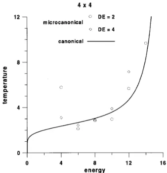
Figure 1. Exact canonical temperature as a function of the energy (continuous line), for a 44 square lattice Ising
ferro-magnet. Symbols correspond to the microcanonical version
of the temperature, equation (8a), with energy gaps E= 2
(circles) or 4 (diamonds).
Fig. 1 showsTm(E) calculated from equation (8a), for a 44 square Ising ferromagnet. The exact val-ues ofg(E) were used. The open circles correspond to E = 2, and the diamonds to E = 4. The contin-uous line is the exact T(E), also calculated from the exact values ofg(E). The deviations between Tm(E) and T(E) are very strong. Note that there is no ap-proximation at all, neither inTm(E) nor inT(E). The deviations represent true dierences between canonical and microcanonical ensembles, which are indeed very strong for this tiny system. Obviously, the condition E << E is not fullled, and the discreteness is in-evitable along the whole energy spectrum.
Fig. 2 reports the same data as Fig. 1, with the same symbols, now for a 3232 lattice, and using equation (8b). The exact values forg(E) were taken from [33]. The same strong deviations occur again, but now only at the very beginning of the energy spectrum, where the condition E << E does not hold, as can be seen in the upper inset. However, near the critical region, the deviations become much smaller, as can be seen in the lower inset where the vertical scale is 100 times ner than the upper one. ForE >64, the energy spectrum discreteness can be neglected within a very good approximation, even with N = 1024 being still very far from the thermodynamic limit in equation (7). The larger the system size, the better becomes the sit-uation, because the relation E << E becomes more and more fullled. However, at the very beginning of the spectrum this relation will never be fullled, even for large systems.
Both limits in equation (7), namely the thermody-namic one N ! 1 and E ! 0 corresponding to the energy derivative, were neglected in equation (8a). However, only the latter seems to have disastrous con-sequences when one uses Tm(E) as an approximation forT(E). Indeed, even for very small systems like the 3232 square lattice (not so tiny as 44), the devia-tions are very small, provided the condition E <<E holds. In other words, the deviations between the mi-crocanonical temperatureTm(E) and the true canonical value T(E) comes almost exclusively from the break-down of the condition E<<E,
not from nite size
eects. Even in the thermodynamic limit,
Tm(E)will dier from
T(E)near the ground state, due
Figure 2. The same as gure 1, now for a 3232 lattice,
with the same symbols, and equation (8b). Note that the deviations between the true canonical temperatures and the microcanonical versions are now restricted to the very be-ginning of the energy spectrum (upper inset). At the critical region these deviations are much smaller (lower inset, with a 100 times ner scale). The deviations become smaller yet for larger systems.
Figure 3. Specic heat for the 3232 lattice Ising
ferromag-net, adopting the random walk dynamics within restricted energy windows [19]. Circles show the exact values [33].
Tables II to VI present good numerical accuracies not only for the tuned temperatures, but also when out-of-tune values for T were considered. Moreover, based on the reasonings above, this feature will be even improved for larger and larger systems. The imediate consequence is the possibility of adding dierent his-tograms for < N
up(
E) > and< N dn(
E) >, obtained from distinct canonical simulations with dierent tem-peratures, as already tested in [17,9]. Of course, this approach is much more ecient than to take a dierent canonical simulation with xed temperature T(E) for each dierent energy level E, without superimposing the histograms. However, it still needs many computer runs, one for each xed temperature.
In order to improve even more the eciency, one can try the following strategy. First, one denes the Boltzmann acceptance probability exp[,E=T(E)]
for
each energy level
E and each possible energy jump E. Note that this is not the same as canonical simu-lations where the acceptance probability exp(,E=T) depends only on E butnot on
E. Then, by follow-ing this non-canonical,E-dependent acceptance proba-bility, one runsa single
computer simulation, visiting the whole energy axis, accumulating the histograms for <Nup(
E)>and<N dn(
E)>. This approach is sim-ilar to the at histogram dynamics [27], using the true temperature T(E) instead of the microcanonical value Tm(E). Table VII shows the results for the same tiny system already considered before. Surprisingly, strong deviations appear. In order to analyse the source of these deviations, let's introduce another very similar alternative, adopting a dierent acceptance probabil-ity exp[,E=T(E + E=2)]. The canonical Boltz-mann probability is taken
at the center
E+ E=2 of the interval correponding to the energy jump from E toE+ E, not at the current energyE. This sym-metrization trick is supposed to diminish the numerical deviations due to impossibility of performing the limit E!0, i.e. the derivative in equation (7), for this tiny system. The results are shown in Table VIII, in com-plete agreement with the exact results, Table I. Thus, the source of the deviations in Table VII is the lack of the condition E << E. By taking into account both the current energy level E as well as the (would-be) next energy E+ Ein a symmetric way
, the numerical deviations were eliminated. Of course, for larger systems and far from the ground state, where the condition E<<Eholds, the dierences between Tables VII and VIII would also disappear.The at histogram dynamics uses another accep-tance probability, namely
c exp[,E=Tm(E)] =
g(E) g(E+ E) =
<N dn(
E+ E)> <N
up( E)>
where E and E+ E also play a
symmetric
role. Simulational results are shown in Table IX, where the exact values for g(E) (or, alternatively, < Nup( E) > and <N
dn(
E)>) were adopted in order to determine the acceptance probabilities (9). The results are again coincident with the expected ones, Table I [34]. On the
other hand, if one tries to break the quoted symmetry, ignoring E in the numerator of the right-hand-side term in (9), i.e. approximation A2, numerical devia-tions similar to Table VII would appear, for this tiny system.
As one does not know a priori g(E) (or, alterna-tively,<N
up(
E)>and<N dn(
E)>), one can use some previous estimates < N
up( E) >
0 and < N
dn( E) >
0, and adopts the acceptance probability (6). In order to follow this recipe [27], one needs to determine the quoted estimates from a previous computer run. Ac-cording to [27], these previous estimates do not need to be very accurate. However, actual numerical tests [29] show results for <N
up(
E)> and <N dn(
E) >worse than the inputs<N
up( E)>
0and <N
dn( E)>
0 them-selves! A better possibility is the random walk dynam-ics originally used in order to test the broad histogram method [1]. It is the same as the at histogram, equa-tion (6) or (9), with the approximaequa-tion A1 (opequa-tionally, also A2 and A3) quoted in last section. A1 consists in taking the current, already accumulated values of the histogramsN
up(
E) andN dn(
E+E), in real time during the computer run itself, instead of the true av-erages at the right-hand side of equation (6) or (9). Re-sults for the same tiny system treated before are shown in Table X. This approach is the same as the multi-canonical retime-measured transition probability al-ready adopted in other earlier methods, for instance
the entropic sampling [6]. A criticism to this approach is its non-strictly-Markovian, history-dependent char-acter. According to [29], it is actually better than the xed transition probability proposed in [27]. Approxi-mation A2 consists in neglecting E in the numerators of equation (6) or (9), breaking the symmetry between levels E and E+ E, and cannot be applied to this tiny system due to the spectrum discretness. This ap-proach A2 is also shown to violate a particular detailed balance condition [27]. A3 consists in taking all pos-sible values for E together, by using equations (5a) and (5b). Both approximations A2 and A3 (but not A1) are bad: a) at very low energies, for any system; b) at any energy, for tiny systems.
The dierence between the dynamics adopted in Ta-bles VII to X and the true canonical rule adopted in Tables II to VI is the following. Canonical simulations adopt
the same
acceptance probability exp(,E=T) for any tossed movement increasing the energy by E, no matter which is the current energy E. As a conse-quence, the energies visited during the run became re-stricted to a narrow window around the canonical aver-age<E>is this window. On the other hand, within the non-canonical rules adopted in Table VII to X, the accep-tance probabilities depend also onE(andE+E). As a consequence, instead of a narrow distribution of visits, one gets a broad distribution covering the whole energy axis. This feature is, of course, a big advantage over canonical rules, because only one run would be enough to cover a large temperature range. Nevertheless, the numerical results could be wrong, depending on the
ac-tual dynamic rule one adopts (Table VII, for instance). A better conceptual, theoretical understanding of these and other E-dependent dynamic rules is needed, and lacking. Concerning BHM, the only constraint to be considered is the uniform probability visitation inside each energy level, separately. For other, reweighting methods based on the actual visitation prole V(E), also the detailed relative distribution between dierent energy levels must be considered.
Up to now, we have tested many dierent dynamic rules in order to measure the microcanonical averages < N
up(
E) > and < N dn(
E) > from which one can determine the desired quantityg(E) by BHM equation (4). The most ecient approaches are theE-dependent rules (Tables VIII, IX and X), where a single computer run is enough. Among them, under a practical point of view, the random walk dynamics [1] corresponding to Table X is the best choice, once one does not need any previous knowledge about the quantities < N
up( E) > and <N
dn(
E)>to be measured. This approach cor-responds to approximation A1. The other two further approximations A2 and A3 [1] improve even more the eciency. However, due to the energy spectrum dis-creteness, they are limited by the constraint E<<E: one needs to avoid them for tiny systems, or very near the ground state even for large systems, where this con-straint cannot be fullled. All this matter corresponds to the subject discussed in reference [27]. Let's now
discuss another, subtle, further possible source of unac-curacies, which may appear when one abandon the safe canonical dynamical rules and adopts non-canonical, E-dependent dynamics in order to sample the whole energy axis during the same computer run.
In order to introduce the subject, let's resort again to canonical simulations,where some temperature value T is xed since beginning. Imagine one starts such a simulationalprocess from a randomlychosen microstate S: its energy E
S would be in general far from the av-erage value<E >
T, as well as many other features of this microstate which would be far from their equilib-rium counterparts. By plotting the energy of each suc-cessive averaging microstate as a function of the time, one would get a curve uctuating around an exponen-tial decay to the nal value<E>
nal averages < Q >T. These are the so-called ther-malizationtransient steps. Nevertheless, they represent no problem at all, because one can always take an enor-mous number of microstatesafterthis transient bias is already over, pushing the systematic deviations to be-low any predetermined tolerance. Better yet, one can simply discard the contribution of these initial states, by starting the averaging procedure only after the tran-sient is over. In the statistical physicists' jargon, one can assert that \the system is already thermalized", af-ter these initial out-of-equilibrium, transient steps.
As quoted in [27], detailed balance is a delicate mat-ter. Detailed balance conditions are useful only in or-der to ensure that the nal distribution, chosen by the user, will be the correct one, for instance the Gibbs distribution for equilibrium canonical averages. How-ever, these conditions do not ensure this nal distri-bution will be reached within a nite time. In our case of interest, i.e. the E-dependent, broad-energy, non-canonical dynamics, the system never reaches canonical equilibrium inside each energy level. All these dynamic rules correspond to generalized Boltz-mann factors exp[,E=(E)], where the \tempera-ture" (E) varies from one microstate to the next, along the Markovian chain. Concerning the energy, for instance, instead of an exponential decay to the canoni-cal equilibrium situation, one gets a random walk visit-ing allenergies, with uctuations coveringthe whole energy axis all the time. The same large uctua-tion behaviour holds also for other quantities, in par-ticular the one for which the microcanonical averag-ing is in progress. This dynamics follows an eternal transientin what concerns the safe canonical frame-work. This feature may introduce systematic numerical deviations. Although those possible out-of-canonical-equilibrium problems cannot be observed in our Tables VIII, IX and X, they could be crucial for larger systems where large energy jumps in few steps become possible: features of a particular far energy region which the sys-tem recently cames from could introduce biases in the current energy averages. In this eternal-transient case, detailed balance conditions and all the related theorems give little help. To construct a good, ecient micro-canonical simulator, by visiting the whole energy axis during a single computer run, seems to be a much more delicate matter. How to assure a uniform probability distribution inside each energy level also covering broad regions of the energy spectrum? This problem is open to new insight, new ideas.
Exemplifying how dicult would be to analyse the uniformity of visits within each energy level, let's take a simple example: a LL square lattice Ising magnet (L > 4, N = L2 spins), with E = 8. Considering the magnetization density m, level E = 8 is divided into three classes. The rst one contains g1(8) = N(N
,5) states with only two non-neighbouring spins pointing
down (all other spins up, or vice-versa), correspond-ing to m = 1,4=N. The second class consists of g2(8) = 12N states with a 3-site cluster of neighbour-ing spins pointneighbour-ing down, with m = 1,6=N. The third class has g3(8) = 2N states presenting a plaquette of four spins pointing down, and m = 1,8=N. No single-spin ip can transform a state with E = 4 or E = 6 into another state belonging to this third class, for in-stance. In order to assure a uniform distribution of visits, this lack must be compensated by other possi-ble single-spin ips from E = 10 and E = 12. On the other hand, the visitation frequency to each one of these higher-energy states depends on feeding rates from higher yet energies, and so on. One must prescribe adequate transition probabilities to each such move-ment, taking into account all its consequences on the next, next-next step, and so on. Chessboard is an eas-ier game. Fortunately, the rst class containingN
2 states dominates the counting for large lattice sizes. For L = 32, for instance, g1(8) = 1;043;456 states are in the rst class, representing 99% of the whole number g(8) = g1(8) + g2(8) + g3(8) = 1;057;792. Similar behaviours also occur for higher energies, giving us a solace: we remain with the hope that single-spin ips may lead to the desired uniformity for large enough sys-tems. For a tiny 44 lattice, on the other hand, things go worse, once two further classes must be added to E = 8 level: g4(8) = 16 states with a single line of spins down, corresponding to m = 1=2; and g5(8) = 8 states with two neighbouring lines of spins down, with m = 0. Then, only g1(8) = 176 states out of g(8) = 424, i.e. 42%, belong to the rst class. This feature, of course, partially explains the bad results in Table VII. However, a detailed explanation for the good results obtained in Tables VIII, IX and X, following the same reasonings, is not easy.
V Improved Microcanonical
Simulators
systems present a plateau of almost constant tempera-tures covering a large energy range. This range is just the interesting one, namely the critical region where the specic heat diverges for N ! 1. Third, with small variations of the temperature from one microstate to the next, within this region, the out-of-canonical-equilibrium problems should be strongly diminished.
Anyway, we can try to introduce some repairing pro-cedures into the random walk dynamics [1] (or into any otherE-dependent transition rate dynamics). The rst idea is to equilibrate the system before measuring any averaging quantity at the current microstate. This can be acomplished by running some canonical steps just before the measuring procedure. Suppose one gets some microstate with energy E, during the random walk dynamics. As this microstate comes from other en-ergy levels, submitted to acceptance probabilities oth-ers than the currently correct value exp[,E=T(E)], it is supposed to carry some undesired biases. Then, one can simply include some canonical steps with xed temperature T =T(E), in order to let the system re-lax toE-equilibrium, before taking the averages. T(E) can be estimated at each step from the current, already accumulated histograms for N
up(
E) andN dn(
E) (ap-proximation A1), and the further ap(ap-proximations A2 and A3 can also be adopted. All these tricks were al-ready introduced in the original publication [1].
Another repairing procedure is simply to forbid large energy jumps. The simplest way to perform this task is to count a new averaging state after each single-spin-ip trial. Normally, one adopts N trials, i.e. a whole lattice sweep, before counting a new averaging state, in order to avoid possible correlations along the Markovian chain of states. In our microcanonical case, however, dierent energy levels correspond to indepen-dent averaging processes, and one can try to abandon this precaution. Of course, this approach also saves a lot of computer time. Table XI shows the results obtained for a 3232 lattice, where approximation A1 (real-time measurement of the transition rates) was adopted, with 109 averaging states per energy level. The expected relative error due to nite statistics is thus 310
,5. Indeed, the observed deviations coincide with this, in spite of the gure 0:008 [27] predicted by detailed balance arguments. Even adopting the further approximations A2 (which explicitly violates detailed balance) and A3, the errors remain the same (last col-umn). Once more, the possible source of unaccuracies has nothing to do with detailed balance dictating the relative frequency of visits between
dierent energy
levels
. On the contrary, the only crucial point is the uniformity of visitsinside each energy level,
sepa-rately
.Perhaps the procedure of measuring averages after each new single-spin-ip trial could indeed introduce some bias, through some undesirable correlations along the Markovian chain, although this possibility is not apparent at all in Table XI. Perhaps this bias could ap-pear only for much larger statistics. An alternative way to avoid large energy jumps still taking averages only after each whole lattice sweep is to restrict the random walk to narrow energy windows. This corresponds to the Creutz energy-bag simulator [24] combined with the random walk dynamics [1] inside each window. It was introduced in [19], and the results also show relative er-rors much smaller than those predicted by detailed bal-ance arguments. The specic heat for a 3232 square lattice is shown in gure 3, where approximations A1, A2 and A3 were used. By restricting the energy to nar-row windows, one is also restricting the temperature to small variations, thus forcing the system to be always near the canonical equilibrium conditions for any en-ergy inside the current window. Once again, the best performance occurs at the critical region.
VI - Conclusions
The Broad Histogram Method (BHM) introduced in [1] allows one to determine the energy spectrum of any system, i.e. the degeneracy g(E) as a function of the energy E, through the
exact and completely
gen-eral
equation (4). First, one needs to adopt some re-versible protocol of allowed movements in the system's space of states. Reversible means that for any allowed movementS !S0, the back movement S
0
!S is also allowed. For Ising models, for instance, one can choose single-spin ips, to ip clusters of neighboring spins, etc. In fact, one could invent
any
protocol. For each state S, Nup
S counts the number of such allowed move-ments for which the system's energy would be increased by a
xed
amount E. Accordingly, Ndn
S counts the number of allowed movements decreasing the energy by
the same
amount E. The energy jump E is also chosen and xed since the beginning. <Nup(
E)>and <N
dn(
By following the same way adopted in measuring < N
up(
E) > and < N dn(
E) >, one can also obtain the microcanonical average<Q(E)>of the particular thermodynamic quantityQof interest (magnetization, density, correlations, etc).
All
these microcanonical averages areindependent
of the particular environ-ment the system is currently interacting with. In other words, they do not depend on temperatures, equilib-rium conditions, or any other thermodynamic concept: they are determined by the system's energy spectrum alone. Thus, after g(E) is already determined through the BHM equation (4), once and forever, the same sys-tem can be submitted to dierent environment condi-tions, and its behaviour (equilibrium or not) can be studied resorting always to the sameg(E). Within the particular case of canonical equilibrium, for instance, the thermal average < Q >T of the quantity Q can be obtained from equation (3), for any temperature T. If one decides to use computer simulations as the in-strument measuring < N
up(
E) >, < N dn(
E) > and < Q(E)>, then only one computer run is enough to determine the whole temperature dependence, contin-uously, without need of repeating again the simulation for each new temperature.
Other computer simulation methods, the so-called multicanonical sampling strategies [5-7], also allow the direct determination of g(E). All of them are based
on the countingV(E) of visits to each energy levelE. Every time each energy levelE is visited by the cur-rent state S, along the Markovian chain, the count-ing is updated from the current V(E) to V(E) + 1. Within BHM, however, theE-histograms forN
up and N
dnare updated from the current N
up(
E) andN dn(
E) toN
up( E) +N
up S and
N dn(
E) +N dn
S , respectively, for the same current stateS. This corresponds to
macro-scopic
upgrades instead of the mere counting of one more state. Thus, a much more detailed information is extracted from each averaging state withing BHM than any other method, giving rise to much more ac-curate results. Moreover, the larger the system size, the stronger is this advantage, due to the macroscopic character of the BHM quantitiesNup and N
dn. Another advantage of BHM over other methods is its complete independence concerning the particular dynamic rule adopted in order to measure the micro-canonical averages.
Any
recipe can be used, provided the correct E-functions < Nup(
E) >, < N dn(
require-ment to obtain correct microcanonical averages is a uniform probability distribution inside each energy level, separately. Detailed balance between dier-entenergy levelsis irrelevant for BHM. Allpossible transitions between dierent energy levels are exactly counted by the BHM quantities N
up and N
dn them-selves,notby the particular stochastic dynamic recipe one adopts. On the other hand, besides the uniform sampling probability inside each energy level, multi-canonical methods also depend on the particular tran-sition rates between dierent energies, which are tuned during the computer run in order to get a at distri-bution of visits at the end. Detailed balance is funda-mental for multicanonical methods. Thus, besides the acccuracy advantage commented before, any good dy-namic rule for multicanonical sampling is also good for BHM, but the reverse is not true. Indeed, BHM allows the user to design his own prole of visits along the energy axis, taking for instance a better statistics near the critical region.
During the past half century, theoretical studies pro-vided us with many recipes concerning detailed bal-ance for Markovian processes, leading to Gibbs equilib-rium distribution. These recipes show us how to design adequate transition rates between dierent energy lev-els. Unfortunately, there are no equivalent theoretical studies in what concerns adequate rules leading to a uniform probability inside each energy level. Perhaps this missing point is due to the fact that most studies were directed towards canonical distributions, where a sharp region of the energy axis is visited: after some transient steps (normally discarded from the Marko-vian chain) the system becomes trapped into this sharp region. Thus, the spread over this restricted region is supposed to occur naturally, giving rise to the required uniformity inside each level. At least for smooth E -dependent quantities <Q(E)>, the quoted sharpness solves the problem. However, this is not the case if one needs to cover wide energy ranges. For both mul-ticanonical sampling as well as BHM, this is an open problem waiting for new ideas, new insight. How to assure a uniform probability of visits inside each en-ergy level? Some clues towards the answer were dis-cussed, and some very ecient practical solutions were proposed in section V.
Acknowledgements
This work was partially supported by the Brazilian agencies CAPES, CNPq and FAPERJ. I am deeply in-debted to Jian-Sheng Wang for exhaustive and elucida-tive discussions about the subtleties inherent to this matter. These discussions were, at least, very useful in showing me my ignorance about the subject, and perhaps also showing us some possible ways to learn a little bit. I am also indebted to my collaborators Hans Herrmann, Thadeu Penna and mainly Adriano Lima,
the youngest one who nevertheless becames the most expert on BHM.
References
[1] P.M.C. de Oliveira, T.J.P. Penna and H.J. Herrmann,
Braz. J. Phys. 26, 677 (1996) (also in Cond-Mat
9610041).
[2] P.M.C. de Oliveira, Eur. Phys. J.B6, 111 (1998) (also
in Cond-Mat 9807354).
[3] Z.W. Salzburg, J.D. Jacobson, W. Fickett and W.W. Wood, J. Chem. Phys.30, 65 (1959); R.W. Swendsen,
PhysicaA194, 53 (1993), and references therein.
[4] G.M. Torrie and J.P. Valleau,Chem. Phys. Lett.28, 578
(1974); B. Bhanot, S. Black, P. Carter and S. Salvador,
Phys. Lett. B183, 381 (1987); M. Karliner, S. Sharpe
and Y. Chang,Nucl. Phys.B302, 204 (1988).
[5] B.A. Berg and T. Neuhaus, Phys. Lett. B267, 249
(1991); A.P. Lyubartsev, A.A. Martsinovski, S.V. Shevkunov and P.N. Vorontsov-Velyaminov, J. Chem. Phys.96, 1776 (1992); E. Marinari and G. Parisi,
Euro-phys. Lett.19, 451 (1992); B.A. Berg,Int. J. Mod. Phys. C4, 249 (1993).
[6] J. Lee,Phys. Rev. Lett.71, 211 (1993).
[7] B. Hesselbo and R.B. Stinchcombe,Phys. Rev. Lett.74,
2151 (1995).
[8] All real systems of interest are conned to a nite vol-ume, thus the energy spectrum will be always discrete. Nevertheless, the method can be easily generalized also for the case of continuous energy spectra models, as in J.D. Mu~noz and H.J. Herrmann, Int. J. Mod. Phys.
C10, 95 (1999); Comput. Phys. Comm. 121-122, 13
(1999).
[9] J.-S. Wang, T.K. Tay and R.H. Swendsen, Phys. Rev. Lett.82, 476 (1999).
[10] G.R. Smith and A.D. Bruce, J. Phys. A28, 6623
(1995); Phys. Rev. E53, 6530 (1996); Europhys. Lett. 39, 91 (1996).
[11] J.-S. Wang and L.W. Lee, Cond-Mat 9903224. [12] M. Kastner, J.D. Munoz and M. Promberger,
Cond-Mat 9906097.
[13] R.H. Swendsen, J.-S. Wang, S.-T. Li, C. Genovese, B. Diggs and J.B. Kadane, Cond-Mat 9908461.
[14] J.-S. Wang, Comput. Phys. Comm. 121-122, 22
(1999); Cond-Mat 9909177.
[15] A.R. de Lima, P.M.C. de Oliveira and T.J.P. Penna,
Solid State Comm.(2000) (also in Cond-Mat 9912152). [16] Energy E = 2 is not allowed, because one cannot
ar-range the spins on the square lattice in such a way that only two unsatised links appear. The same occurs also forE= 2L
2
,2. Besides these two cases, any even value
ofE in between 0 and 2L
2 is allowed.
[17] P.M.C. de Oliveira, T.J.P. Penna and H.J. Herrmann,
Eur. Phys. J. B1, 205 (1998); P.M.C. de Oliveira,
in Computer Simulation Studies in Condensed Matter Physics XI, 169, eds. D.P. Landau and H.-B. Schuttler,
[18] P.M.C. de Oliveira,Int, J. Mod. Phys. , 497 (1998). [19] P.M.C. de Oliveira, Comput. Phys. Comm. 121-122,
16 (1999), presented at the APS/EPS Conference on Computational Physics, Granada, Spain (1998). [20] H.J. Herrmann, J. Stat. Phys. 45, 145 (1986); J.G.
Zabolitzky and H.J. Herrmann,J. Comp. Phys.76, 426
(1988), and references therein.
[21] S.C. Glotzer, D. Stauer and S. Satry, PhysicaA164,
1 (1990).
[22] C. Moukarzel,J. Phys.A22, 4487 (1989).
[23] M. Schulte, W. Stiefelhaben and E.S. Demme,J. Phys.
A20, L1023 (1987).
[24] M. Creutz,Phys. Rev. Lett.50, 1411 (1983).
[25] C.M. Care,J. Phys.A29, L505 (1996).
[26] B. Berg,Nature361, 708 (1993).
[27] J.-S. Wang,Eur. Phys. J.B8, 287 (1999) (also in
Cond-Mat 9810017).
[28] B. Berg and U.H.E. Hansmann,Eur. Phys. J.B6, 395
(1998).
[29] A.R. de Lima, P.M.C. de Oliveira and T.J.P. Penna,J. Stat. Phys.(2000) (also in Cond-Mat 0002176).
[30] J.L. Lebowitz, J.K. Percus and L. Verlet,Phys. Rev.
153, 250 (1967); D.H.E. Gross, Phys. Rep. 279, 119
(1997), and references therein; D.H.E. Gross, Cond-Mat 9805391; M. Kastner, M. Promberger and A. Huller, in Computer Simulation Studies in Condensed Mat-ter PhysicsXI, eds. D.P. Landau and H.-B. Schuttler,
Springer, Heidelberg/Berlin (1998); M. Promberger, M. Kastner and A. Huller, Cond-Mat 9904265.
[31] N. Metropolis, A.W. Rosenbluth, M.N. Rosenbluth, A.H. Teller and E. Teller, J. Chem. Phys. 21, 1087
(1953).
[32] P.M.C. de Oliveira, T.J.P. Penna, S. Moss de Oliveira and R.M. Zorzenon,J. Phys.A24, 219 (1991); P.M.C.
de Oliveira, Computing Boolean Statistical Models, World Scientic, Sigapore London New York, ISBN 981-02-0238-5 (1991).
[33] P.D. Beale,Phys. Rev. Lett.76, 78 (1996).
![Figure 3. Specic heat for the 32 32 lattice Ising ferromag- ferromag-net, adopting the random walk dynamics within restricted energy windows [19]](https://thumb-eu.123doks.com/thumbv2/123dok_br/18979205.456402/10.918.112.459.594.963/figure-specic-lattice-ferromag-ferromag-adopting-dynamics-restricted.webp)
