J. Microw. Optoelectron. Electromagn. Appl. vol.12 número2

(1)

Brazilian Microwave and Optoelectronics Society-SBMO received 21 Oct 2012; for review 7 Dec 2012; accepted 5 July 2013

Abstract— Direct capture of carriers from the wetting layer to the most confined states is discussed in this paper. This channel for carrier scattering was recently used to fit typical P-I curves of quantum dot lasers. Here new numerical expressions for the escape times accounting for the carriers added by the direct channel are introduced and evaluated, and insights of the influence of these additional carriers on the continuous and pulsed laser emission spectrum are given.

Index Terms— Direct capture, direct modulation, quantum dot laser. I. INTRODUCTION

Semiconductor quantum dot (QD) lasers have been intensively studied in the last years because of their potential compared to quantum well and bulk lasers, as well as due to the particular properties associated with the 3D confinement in the quantum dots. As an example, the two-state emission, i.e., simultaneous emission from the fundamental ground (GS) and the first excited state (ES1) in a certain current range has been demonstrated in [1] at different temperature and operating conditions (continuous wave, pulsed regime) and for various cavity lengths. Such phenomenon has been exploited by [2] to produce broad band light sources. In this two-state lasing regime, increasing the injected current leads to suppression of the GS power, and the laser emits from the ES1 only at higher injection levels. This switching from GS to ES1 emission wavelength was, at first, reported in [3] and justified later with the use of simple numerical models. In [4], on the basis of a non-excitonic 2 level (GS,ES1) rate equation system the GS switch-off was explained in terms of the asymmetry between electron and hole population redistribution in the dot states.

That model, however did not consider the inhomogeneous dot size distribution, which is a natural consequence of the Stranski-Krastanow method for growing QDs and, besides, the presence of the wetting layer (WL) medium coupling the various QD groups was neglected. Furthemore, it was not taken into account the existence of the second ES (ES2), which is usually present in devices emitting

at 1.3μm. In [5] a multi-population rate-equation model (MPRE) taking into account the inhomogeneous dot size distribution and the homogeneous gain broadening was used to fit continuous wave (CW) power spectra and explain the transition from GS only to ES1 emission only, with the assumption that GS and ES1 homogeneous broadening linewidth increase linearly with the injected current. Similar assumption was also used in [6] to evaluate and compare the linewidth enhancement

Rate-equations based model for the 2D-0D

direct channel in quantum dot lasers under

CW and gain-switching

George A. P. Thé

(2)

factor of broad band QD lasers with that of typical QD devices. A further simplification of several of these models consists on neglecting the hole dynamics, assuming it mirrors the electron dynamics (excitonic model [7]). Another simplification of the models currently in use in the literature concerns the relaxation path of the injected carriers. After being injected in the higher energy states, the carriers can relax down to the next lower level only. For example, in a dot system with 3 confined states (GS, ES1 and ES2) carriers in the WL are captured in the ES2 and then relax down to the ES1; therefore the direct scattering from the WL to the ES1 is not considered. Although this cascaded relaxation model is universally used to simulate QD lasers [8], [9], [10], [11], several theoretical and experimental works have reported the existence of a direct capture of carriers from the two dimensional carrier reservoir to the GS and to the ES1 [12], [13], [14]. Despite of this, very few works have included such phenomenon in the rate equations (RE) system because in the scenario of cascaded relaxation the escape times can be easily calculated from analytical expressions [15].

Recently a laser RE model accounting for the direct capture of electrons from the WL to GS and to ES has been used to fit the gradual suppression of the GS CW power which occurs after the appearance of the ES1 lasing line [16], but no detailed description of the model has been done yet. Such a model is described in the present work and new expressions for the escape times are introduced. This paper is organized as follows: in the next section the non-excitonic model with the inclusion of expressions for the carrier escape times is presented, and these new equations are numerically checked. In section III the influence of the direct capture on the emission spectrum is discussed and new insights into the pulsed regime are given, including discussion of the frequency chirp at different modulation rates and estimate of an equivalent linewidth enhancement factor from the adiabatic chirp coefficient. Finally, conclusions are drawn.

II. MODELING AND DISCUSSION

The non-excitonic model here proposed considers that electrons and holes follow different dynamics and, therefore, a set of time-domain carrier number equations is established for electrons, whereas another one is written down for holes. This assumption comes from the expected band diagram of the laser material we are dealing with, which is InAs quantum dots inserted in InGaAs quantum well, with GaAs separate confinement heterostructure (SCH). With the help of NextNano3D simulation tool we designed QD size and quantum well thickness to get emission from the

(3)

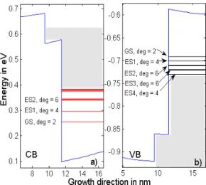
Fig. 1. Band diagram of quantum dot material: a) Conduction Band b) Valence Band.

Carrier dynamics for electrons in conduction band requires, therefore, at least five equations: electron number in the SCH, in the WL, in the ES2, in the ES1 and in the GS. Actually, for properly taking into account the inhomogeneous dot size distribution, it is considered that quantum dots of an ensemble are separated into n small groups of dots similar in size; this leads to n equations for carrier number of each confined state (GS, ES1 and ES2). See [8] for details on such multi-population formulation. For what concerns the valence band, Fig. 1b, five confined states almost equally separated (about 15 meV) have been found. The upper continuum is indicated with the shaded area and correponds to the WL states of the holes. Due to the larger effective mass, energy states for holes are separated by less than the thermal energy at room temperature. Furthermore, being the hole dynamics much faster than the electron dynamics, it is assumed that the holes are always in quasithermal equilibrium within the confined states and the upper continuum. Therefore the hole distribution versus energy is always given by a Fermi-Dirac function characterized by a quasi-Fermi level that allows satisfying the neutrality condition [15].

Under this assumption, the rate equations for the holes in VB reduce to two: one equation for holes

in the SCH, and one for the total number of holes in the “dot states”., i.e., the ensemble of states

formed by the WL plus the states with three dimensional confinement in the QD (GS, ES1...ES4). A. Rate equations

Traditionally, in a rate-equation approach for laser simulation time-variation of carrier number is given as the contribution of several carrier scattering phenomena that lead to relaxation, escape, diffusion and recombination processes. For the sake of simplicity, recombination terms are omitted in the forthcoming equations since they do not take place in the derivation of the formulae of next section. Terms related to the direct scattering 2D-0D are in bold type in the following equations.

ws w

sw s s

t n + t

n e I =

(4)













w0 w w1 w w2 w ws w sw s w t

ρ

n t

ρ

n t

ρ

n t n t n + t n =

n





1 

2





1 

1





1 

0

2w 2



(2)













2w 2 2 21 1 2 12 2 1 2

1

t n t

ρ

n + t

ρ

n t

ρ

n = n w2 w













₍₃₎





















10 0 1 12 2 1 01 1 0 21 1 2 1

1

t

ρ

n t

ρ

n t

ρ

n + t

ρ

n + t

ρ

n = n w1

w



















1



(4)













01 1 0 10 0 1 0

1

t

ρ

n t

ρ

n + t

ρ

n = n w0

w











0



₍₅₎

They are written according to the carrier dynamics in CB, sketched in Fig.2. Carriers are injected into the SCH and, then, diffuse to the WL reservoir according to a rate 1/tsw. They can be captured in the ES2 and follow a cascaded relaxation down to ES1 and to GS. This cascaded relaxation path is indicated with solid arrows in Fig. 2. Alternatively, the carriers in the WL can follow the direct capture path from the WL directly to the ES1 or to the GS. These direct capture paths, indicated with dashed arrows in Fig. 2 are included in the rate-equations with rates 1/tw1 and 1/tw0. The time constants for the capture times have been calculated theoretically in [12] and measured by time-resolved photoluminescence experiments in [13], [14]. With solid-curved arrows in Fig. 2 the escape processes due to carrier thermalization are illustrated. It is assumed that the escape can occur only from one state to the upper one (i.e.: from GS to ES1, from ES1 to ES2). Other escape paths (e.g. from GS or ES1 directly to WL) are less likely because they require the existence of WL carriers at high energy to scatter with [12]. This would require high occupation of WL states, which in turn would be achieved with very high injection conditions not used here.

Fig. 2. Schematic diagram of carrier dynamics in Conduction Band. In dashed arrows the 2D-0D capture channel. In the VB things are simpler, since hole dynamics is governed by two equations only: one for the dot states (index d) and one for holes in the SCH (index s):

ds d sd s s t n + t n e I =

n  (6)

ds d sd s d t n t n =

n  (7)

B. Derivation of escape times

(5)

calculation of the escape times appearing in the system rate equations (t01 and t12, for instance). The escape time terms must lead to a quasi-Fermi distribution of the carriers in steady state and in absence of any carrier generation/loss. This means that, in order to calculate the escape time from GS to ES1 in CB, for example, it is imposed dn0/dt = 0, and all the recombination terms are neglected: stimulated and spontaneous emission and non-radiative processes, as well (here is why they have been omitted previously); in these conditions the filling rate into the GS equals the escape rate out of it, and the escape time can be derived as:









1 1 10 10 0 1 1 0 01

1























w0

w t N t N + t

ρ

N

ρ

N = t (8)

Note that with this notation the carrier number with capital letters in equation (8) indicates the carrier number calculated from a given quasi-Fermi energy, and not the value given by the rate equations at every time instant (see later explanation). Analogously other time expressions can be obtained, respectively escape from ES1 and from ES2:













1 1 2 21 0 2 21 21 1 2 2 1 12 1 1 1 1 1                    w0 w w1 w t ρ N t ρ N + t N t N + t ρ N ρ N = t (9)













1 2 0 2 1 2 2 2w

1

































w0

w2 w1 w2 w w2 t

ρ

t

ρ

+ t

ρ

t

ρ

+

ρ

N t N = t (10)

From these equations one should notice that the escape times depend on the number of carriers in the states involved in the transition and no more on the sole energy separation between the states, as it is true in the Boltzmann limit [15]. Equations (8) to (10) agrees with the values obtained from the literature for the case of only cascaded relaxation, after properly setting tw0 and tw1 to infinite. The reader should realize that with these equations in hand it is straightforward to simulate both cascaded and direct capture relaxation models.

(6)

 

       

 

v F

π

N D H

π

Tm K + T K E E e +

π

D m T K + T K E E e + + T K E E e + + T K E E e + = t n + t n + t n + t n + t n

la yer s d s eff s B B F w d eff w B B F B F B F w s 2 / 1 2 / 3 2 2 2 2 1 1 0 0 0 1 2

2

1 log

1

1 

























































































(11)

where the first part is the sum over the quantum dot population (0D states), the second one is related to the 2D population (WL) and the last one accounts for the carriers in the SCH (3D states). The term F1/2(v) is the Fermi-Dirac integral of order 1/2. A plot of the contribution of each of these terms to the whole carrier population is given in Figure 3 below. Inverting the equation above allows one to find the quasi-Fermi level EF(t) that, if inserted in the equations (8)-(10) gives the escape times at instant t.

Fig. 3. Fermi level as a function of the total number of carriers per dot in the CB (solid line) and in the VB (dotted). In the dashed line, the number of holes per dot in the dot states (SCH excluded). Positive value of the Fermi level represents the

quasi-Fermi level for the electrons, whereas the negative values is for the quasi-Fermi level of the holes.

(7)

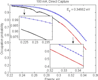
generation/loss terms. The accordance (cross markers and thin line) confirms that the rate equations are correctly balanced, otherwise the thermal distribution would not be achieved through numerical integration.

Fig. 4. Occupation probability at steady state of a quantum dot ensemble under lasing, obtained from solution of rate equations including direct capture relaxation processes (thick line). Thin solid line is the plot of Fermi-Dirac function. Cross

markers indicate the occupation probability from rate equations in absence of generation/loss terms.

III. LASER OPERATION

The model just presented has been successfully used to fit experimental P-I curves and also switch-on transient respswitch-onses of quantum dot lasers [16], for several injectiswitch-on cswitch-onditiswitch-ons and at different temperatures, as well. Here readers are provided with valuable insights on continuous-wave and pulsed operation of quantum dot laser.

A. Power emission spectrum

(8)

The existence of such double emission line in quantum dot based light sources may find useful applications. For instance, broadband incoherent sources have been realized by using the whole emission range from GS to ES, with particular application to optical coherence tomography. Such two-state emission also appears as a function of the laser operating temperature. In fact, temperature gradients of 25oC led to transition from GS emission only to ES emission only [16], and may be exploited to produce temperature tunable light sources, for example.

Fig. 5. On top: cut-section of the emission spectrum around GS and ES lines. In the bottom: net modal gain spectrum dependence on the driving current.

B. Pulsed operation

To further analyze the double-state emission feature, in this section pulsed operation is studied. The objective here is to investigate the features of the optical pulses obtained after large-signal modulation, and see if the direct captured carriers play a role on this, by simulating the same device formerly used under different gain-switching scenarios. The modulation is such that the bottom current is near threshold and the top current is many times that value. The duty cycle has been set to 350 ps and the top current to 250 mA, whereas the repetition rate changed up to 1.5 GHz. In all the simulations, we observed the following pulse properties: peak power, full-width at half maximum, energy ratio and extinction ratio. The energy ratio has been calculated through the following formula:

 

















dt t P

dt t P =

E

GS ES

r

10 log

(12)

where the excited and ground-state power are integrated over the square-wave period, T. The extinction ratio represents the on-off power relation. It is, therefore, a kind of suppression ratio of bit 1 to bit 0, in a base-band communication, calculated as in the following:



















T =

t P

t = t P =

Exr fir stPea k

0.99 log

10

(13)

(9)

relaxation path. If analyzed together with the CW results presented in the literature and discussed in the previous section, this allows for a complete comprehension of the influence of this additional path on the laser performance.

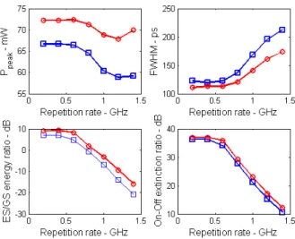
Fig. 6. Parameters of the optical pulses after gain-switching operation as a function of the repetition rate of the modulation current. Comparison of the models including (circle markers) and neglecting (square markers) the direct capture of carriers.

The first result is that the existence of carriers relaxing direct from the wetting layer to ES1 and to GS do not alter qualitatively the optical pulses obtained via gain-switching of quantum dot laser, though it rather influences the CW spectrum. The whole trend with repetition rate is kept practically unchanged in pulsed regime. However, top-left part of Figure 6 exhibits an increase in the peak power (compare red and blue curves). If analyzed together with the bottom-left part of the figure, we conclude this is due to the presence of the spike-like response of photons emitted from ES carrier recombination, which are now stronger than the GS emission (compare red and blue curves to see that ES contributes more to the overall pulse energy when direct channel is added).

Second and more impressive conclusion is also related to the existence of the ES lasing line. If we look at the operating conditions in which excited state emission does constitute a significant part of the optical pulse, i.e., intervals of high energy ratio, we see that higher peak power, shorter optical pulses and higher extinction ratio are achieved. This means that gain-switching is more effective under such conditions. Therefore, for efficient gain-switching operation of quantum dot lasers, look for a scenario in which carriers at excited state contributes more than carriers at ground state as, for instance, low-repetition rate conditions. It should be mentioned that under high-injection current condition similar conclusions apply.

(10)

C. Spectrally resolved optical pulses

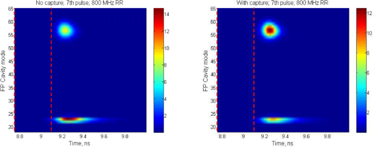
In order to get more insight into the photon dynamics in such multi-mode laser, in Figure 7 the temporal view of the 7th optical pulse of a 800 MHz repetition rate electrical driving is spectrally resolved and shown for both the cascaded only and direct capture models. Note how the rising and trailing edges of the optical pulse are dominated by emission of modes resonant with the fundamental state transition (between 20th and 23rd modes), whereas in the middle of the pulse excited state transition plays major role (between 55th and 60th modes), revealing, therefore, a kind of dynamic mode hopping. From the point of view of the instrumentation in optical detection, such 80 nm separation between fundamental and first excited state transitions should be considered, and preference to InGaAs based devices should be given due to the wide and flat wavelength range.

Fig. 7. Spectrally resolved along time view of an optical pulse, after 800 MHz electrical driving. Left and right parts correspond, respectively, to the cascaded only and direct capture models. Colorbar indicates optical power in mW. Vertical

dashed lines indicate when the electrical pulse was applied. D. Analysis of frequency chirp

From the point-of-view of optical transmission applications, the use of semiconductor lasers under direct modulation might represent a problem since the existence of frequency chirp could potentially cause distortion of the travelling signal (due to chromatic dispersion of optical fibers). It is therefore important to study this feature of a quantum dot laser. In this section some review on this topic is done, the calculation of lasing frequency fluctuation in quantum dot lasers is presented and an expression for equivalent linewidth enhancement factor (LEF) from simulation results is proposed.

Chirping appears due to the carrier density variation in the laser, which causes refractive index variation and, in consequence, change in the optical cavity length. The change in the refractive index at a given lasing mode energy has mainly two contributions:

(11)

contributes to the refractive index change according to a homogeneous broadening function, D(Ej-Eqdot), in such a way that quantum dots whose transition energies of the fundamental or first-excited states are near the considered lasing energy, Ej, are those which contribute more. This is synthesized through the following expression:

 







j qdot



h qot e

qdot j

QD E = C C p + p D E E

Δn

₁





₂





1 



(14)

where C1 and C2 are physical parameters or constants (see [17] for detailed description).

b) the second contribution is related to the free-carrier accumulation in the 2D and 3D states, and is summarized as follows:

 

2 2

j w w j

s s j ca r r ier fr ee

E Δn k + E Δn k = E

Δn _ (15)

where ks and kw are physical parameters or constants (see [17] for detailed description), ∆ns and ∆nw come from the rate equations (section II.A).

Finally, the frequency chirp can then be calculated as:

 



QD fr ee ca r r ier



r

j

Δn

+

Δn

n

π

E = t

Δ





_



2

(16)

An immediate result which can be generated from these formulae is the chirp variation in the power-frequency plane, as shown in Figure 8. Plot of part a) has been obtained from expression (16) with Ej equal to the transition energy of the fundamental state (about 0.96 eV), in a gain-switching with current modulation from near threshold to 5 times this value and for 2 different repetition rates (0.8 and 1.4 GHz). It reveals the overall lasing frequency fluctuation as the light emission alternates between minima and maxima of output pulses. For completeness, in part b) the chirp variation of the optical mode resonant with the first-excited state is depicted.

Fig. 8. Frequency chirp of cavity modes resonant with GS carriers (top) and ES1 carriers (bottom). Dotted line in the top figure indicates the adiabatic chirp.

(12)

transitions, during the leading edge (LE) and trailing edge (TE) of the pulses, whereas the adiabatic causes 1 bits to blue-shift relative to 0 bits [18]. To see how adiabatic chirp appears in the power-frequency plane, note that the y-coordinate of the right-most point of the graph is greater than the left-most point; such misalignment (very thin dotted line in Figure 8) indicates the existence of the adiabatic chirp. Taking as reference the well-known expression for the chirp in Fabry-Perot bulk lasers [19],

 

_ _ g p p_ p

p

N a Γv + dt dN N π α = t

Δ 1

4 (17)

where Np is the photon density inside the cavity, α is the linewidth enhancement factor and ap = dg/dNp, one can identify the first term inside the brackets as the transient chirp. The second term reveals a linear dependence of the chirp on the photon density, given by the adiabatic chirp coefficient kad = α Г vg ap/(4π), which amounts to 0.0159 GHz/mW in the simulation of the GS lasing line of Figure 8, and 0.0143 GHz/mW in the simulation of the ES1 lasing line (both at 1.4GHz repetition rate). These numbers are easily obtained from the graphs by just calculating the inclination of the line connecting minimum and maximum optical power. Adiabatic chirp coefficients for 0.2 GHz and 0.8 GHz are reported in the table below, as well as the maximum frequency fluctuation of the transient chirp (during the leading and trailing edges of the pulses).

TABLE I.CHIRP PARAMETERS AT DIFFERENT MODULATION RATES Repetition rate

(GHz)

kad (GHz/mW)

GS line

kad (GHz/mW)

ES1 line

ΔυLE (GHz)

GS line

ΔυTE (GHz)

GS line

ΔυLE

(GHz)

ES1 line

ΔυTE

(GHz)

ES1 line

0.2 0.0500 0.0554 8.19 -3.60 8.66 -3.99 0.8 0.0370 0.0378 ---- ---- ---- ---- 1.4 0.0159 0.0143 5.36 -4.36 5.54 -4.53

It can be seen from the table that as the modulation rate increases, the adiabatic chirp reduces and the overall transient chirp, as well. This is consistent with the previous results of Figure 6, which revealed shorter pulse-width at lower repetition rates and, therefore, increased chirp at these rates. Since at these rates ES emission dominates the spectrum, it can be stated that higher chirp is achieved with ES dominant scenario and this is explained due to the higher differential gain at the wavelengths around the ES line.

Although it is clear that eq. (17) can not be used to predict the chirp of the quantum dot laser (rigorously it would require the LEF to be dependent on the output power), it is possible to have an

estimate of an equivalent α valid for certain operating points (when dNp/dt = 0, for instance) by equating the resulting terms of eq. (17) and the adiabatic chirp coefficient:

p g

a d a

Γv

πk

=

(13)

To give an example, considering the lasing threshold as operating point allows one to estimate the

equivalent α = 0.05, at the GS lasing line, 0.96eV (see the LEF spectrum in Figure 9).

Fig. 9. Frequency chirp of cavity modes resonant with GS carriers (top) and ES1 carriers (bottom). Dotted line in the top figure indicates the adiabatic chirp.device undergoes variation of the If compared to the well-knownThe frequency

IV. CONCLUSIONS

A non-excitonic model with modified thermal escape times has been developed to take into account the presence of the direct capture of carriers from the 2D wetting layer reservoir to the 0D dot states, GS and ES1, and study its influence on the laser characteristics. The derived equations for the escape times were shown to be more general than the expressions in the literature, since these last can not apply to a rate equation model with the direct capture process present. Simulations showed that when only the cascaded relaxation is assumed, at increasing current a broadening of the gain spectrum around GS is observed after the ES1 lasing onset, which justifies the gradual increase of GS power and its clamping. On the other hand, the inclusion of the carrier direct capture path was shown to cause the opposite effect, with the gain spectrum getting narrow around GS at increasing DC current, until the emission from GS completely ceases, what is in accordance with many measurements published so far. This was explained in terms of the increased escape rate of carriers from GS, additionally populating ES1 and, therefore, favoring its lasing.

Pulsed operation has also been investigated and revealed that the way to get high-power, short-width pulses and high on-off ratio is to work at injection conditions which favor the ES lasing, i.e., lower repetition rates. Nevertheless, under these conditions there is more chirp (both adiabatic and transient), which is associated to the higher differential gain at the wavelengths resonant with the excited state carriers.

(14)

ACKNOWLEDGMENT

Brazilian agency CNPq supported this work (reference number 482393/2011-4).

REFERENCES

[1] A. Markus, J. Chen, O. G.-L. J. Provost, C. Paranthoen, and A. Fiore, “Impact of intraband relaxation on the performance of a quantum-dot laser,” IEEE J. Select. Top. Quantum Electron., vol. 9, no. 5, pp. 1308– 1314, September/October 2003.

[2] H.S. Djie, B.S. Ooi, X.-. Fang, Y. Wu, J.M. Fastenau, W.K. Liu and M. Hopkinson, “Room-temperature broadband emission of an

InGaAs/GaAs quantum dots laser,” Opt. Lett., vol. 32, 1, pp. 44-46, 2007.

[3] G. Park, D.L. Huffaker, Z. Zhou, O.B. Shchekin and D.G. Deppe,“Temperature dependence of lasing characteristics for long -wavelength (1.3μm) GaAs-based quantum-dot laser,” J. Appl. Phys., vol. 97, pp. 43 523 1–8, 2005.

[4] E.A. Viktorov, P. Mandel, Y. Tanguy, J. Houlihan and G. Huyet, “Electron-hole asymmetry and two-state lasing in quantum dot

lasers,” Appl. Phys. Lett., vol. 87, 053113, 2005.

[5] M. Sugawara, N. Hatori, H. Ebe, M. Ishida, Y. Arakawa, T. Akiyama, K. Otsubo, and Y. Nakata, “Modeling room-temperature lasing spectra of 1.3μm InAs/GaAs quantum dot lasers: homogeneous broadening of optical gain under current injection,” J. Appl. Phys., vol. 97, pp. 43 523 1–8, 2005.

[6] C.L. Tan, Y. Wang, H.S. Djie and B.S. Ooi, “Simulation of characteristics of broadband quantum dot lasers,” Opt. and Quantum Electron., vol. 40, 391, 2008.

[7] P. Dawson, O. Rubel, S. D. Baranovskii, K. Pierz, P. Thomas and E. O. Gobel, “Temperature-dependent optical properties of

InAs/GaAs quantum dots: Independent carrier versus exciton relaxation,” Phys. Rev. B, vol. 72, 235301, 2005.

[8] A. Sakamoto and M. Sugawara, “Theoretical calculation of lasing spectra of quantum-dot lasers: effect of homogeneous broadening of

optical gain,” IEEE Photonics Tech. Lett., vol. 12, 2, pp. 107-109, 2000.

[9] T.-En Nee, Y.-Fen Wu, J.-Chyi Lee and J.-Cheng Wang, “Temperature and excitation dependence of photoluminescence spectra of

InAs/GaAs quantum dot heterostructures,” IEEE Transactions on Nanotechnology, vol. 6, 5, pp.492-496, 2007.

[10] L. Shi, Y. Chen, B. Xu, Z. Wang, and Z. Wang, “Effect of interlevel relaxation and cavity length on double-state lasing performance of

quantum dot lasers,” Physica E, vol. 39, pp. 203–208, 2007.

[11] A. Fiore and A. Markus, “Differential gain and gain compression in quantum-dot lasers,” IEEE J. Quantum Electron., vol. 43, no. 4, pp. 287–294, 2007.

[12] T.R. Nielsen, P. Gartner and F. Jahnke, “Many-body theory of carrier capture and relaxation in semiconductor quantum-dot laser,” Phys. Rev. B, vol. 69, 235314, 2004.

[13] P. Miska, C. Paranthoen, J. Even, O. Dehaese, H. Folliot, N. Bertru, S. Loualiche, M. Senes and X. Marie, “Optical spectroscopy and modelling of double-cap grown InAs/InP quantum dots with long wavelength emission,” Semicond. Sci. Technol., vol. 17, L63, 2002. [14] G. Raino, G. Visimberga, A. Salhi, M.T. Todaro, M. De Vittorio, A. Passaseo, R. Cingolani and M. De Giorgi, “The influence of

continuum background on carrier relaxation in InAs/InGaAs quantum dot,” Nanoscale Res. Lett., vol. 2, 509, 2007.

[15] A. Markus, M. Rossetti, V. Calligari, J.X. Chen and A. Fiore, “Role of thermal hopping and homogeneous broadening on the spectral characteristics of quantum dot lasers,” Journal of Appl. Phys., vol. 98, 104506, 2005.

[16] L. Drzewietzki et al., “Theoretical and experimental investigations of the temperature-dependent continuous wave lasing characteristics and the switch-on dynamics of an InAs/InGaAs quantum-dot semiconductor laser”, Opt. Comm., vol. 283, no. 24, pp. 5092-5098, 2010.

[17] G. A. P. The, Improved modeling and simulation of quantum dot lasers, PhD Thesis, chapter 2, Polytechnic of Turin, Italy, 2010. [18] Z. F. Fan and D. Mahgerefteh , “Chirp managed lasers: A new technology for 10 Gbps optical transmitters”, Optik & Photonik, no. 4,

pp. 39-41, December 2007.