Abstract
Using GDQ method, the radial and circumferential stresses in an annular FGM plate with a uniform thickness under a transverse axisymmetric load is investigated. It is assumed that a uniform radial magnetic field acts on the top surface of the plate. The mod-ulus of elasticity E and the magnetic permeability coefficient
of the plate along its thickness are assumed to vary according to the volume distribution function. The Poisson’s ratio
is consid-ered to be constant. Based on the classical plate theory (CPT), equilibrium equations are deduced and the displacement fields are determined. The radial and circumferential stresses as well as transverse and radial displacements are obtained accordingly. The effect of volume fraction function power m on the maximum deflec-tion in the absence and presence of the magnetic field is also inves-tigated. Moreover, the effect of t/a and b/a ratios on displacements, stresses, induction magnetic field intensity and the resulting Lo-rentz force are also investigated. According to the results, for dif-ferent points along the radial direction, the application of radial magnetic field to the top surface of the plate completely changes the state of stress in both tangential and radial directions, resulting in tensile and compressive stresses in these two directions. The results also indicate that in presence of magnetic field, the plate displacement and stress components are lowered considerably.Keywords
Functionally Graded Material, Magneto Elastic, GDQ method
Magneto-Elastic Analysis of an Annular FGM Plate
Based on Classical Plate Theory Using GDQ Method
1 INTRODUCTION
Functionally graded materials (FGM) are heterogeneous composites which are usually a com-bination of ceramic and metal, or a comcom-bination of two or more different metals. Properties of FG materials change uniformly and continuously across the thickness, from point to point,
M. Shishesaz a A. Zakipour b A. Jafarzadeh c
a Department of Mechanical Engineering,
Shahid Chamran University of Ahvaz, Ahvaz, Iran
E-mail address: [email protected]
b Mechanical Engineering Department,
Islamic Azad University, Behbahan Branch, Behbahan, Iran
E-mail address: [email protected] c Mechanical Engineering Department,
Amirkabir University of Technology, Tehran, Iran
E-mail address: [email protected] http://dx.doi.org/10.1590/1679-78252880
according to a function. These materials can be used when good thermal and mechanical re-sistances are required simultaneously. For example, in a FGM plate made of ceramic and metal, the ceramic sector is a good insulator against heat and thermal shocks while the metal-lic sector acts as a good resistance against mechanical loads. The unique properties of these materials are due to their composite nature and their physical properties which gradually change across the thickness of the specimen. This in effect reduces the hysteresis stresses, as well as the stress concentration, with a significant improvement in mechanical properties of the overall material, especially at the ceramic and metallic junction.
In recent years, considerable research has been oriented toward FGM plates to better un-derstand their behavior under various loading conditions. Bayat et al. (2014) investigated the magneto-thermo-mechanical response of a FGM annular rotating disc with variable thickness and observed that unlike the positive radial stresses developed in a mechanically loaded FGM disk, in a FGMM (functionally graded magneto-elastic material) disk, the radial stresses due to magneto - thermal load can be both tensile and compressive. Behravan Rad and Shariyat (2015) analyzed a porous circular FG plate with variable thickness subjected to non-axisymmetric and non-uniform shear along with a normal traction and a magnetic actuation. The plate was supported on a non-uniform Kerr elastic foundation. They evaluated the effect of material, loading, boundary and elastic foundation on the resulting displacement, stress, Lorentz force, electromagnetic stress and magnetic perturbation quantities. Chi and Chung (2006) studied the mechanical behavior of FGM plates under transverse load using a numeri-cal method. Ma and Wang (2003) studied nonlinear buckling and bending behavior of FGM circular plates under mechanical and thermal loads based on the classical nonlinear von Kar-man plate theory. They discussed the effects of material power distribution function and boundary conditions on the temperature distribution, nonlinear bending, critical buckling temperature and thermal post-buckling behavior of the plate in details. Najafizadeh and Hey-dari (2004) analyzed thermal buckling of FGM circular plates under various thermal loads based on higher order shear deformation theory (HSDT) and compared their results with those obtained using first order shear deformation theory (FSDT) and classical plate theory (CPT). They showed that HSDT theory predicts the behavior of FGM circular plates with higher precision compared to FSD and CP theories. Praveen and Reddy (1998) studied the thermo elastostatic and thermo-elastodynamic response of FGM plates subjected to varying pressure and temperature loading. They showed that the combination proportion of materials in FGM plates plays an important role on determining their response. Reddy et al. (1999) analyzed axisymmetric bending and stretching of FGM annular plates using the first-order shear deformation Mindlin plate theory and concluded that this theory gives good results on FGM annular plates whenever the Kirchhoff solution is not applicable.
for magneto dynamic stress and perturbation response of an axial magnetic field vector in an orthotropic cylinder under thermal and mechanical shock loads. They deduced the response histories of dynamic stresses and the perturbation of the field vector. Yuda and Jing (2009) obtained the electrodynamic equations and electromagnetic force expressions of a current-conducting thin plate in an electromagnetic field, based on Maxwell equations. They investi-gated the nonlinear sub-harmonic resonance of the thin plate with two simply supports on opposite sides under a mechanical live load. In their analysis, an inconstant transverse mag-netic field load was applied as well.
Ghorbanpour Arani et al. (2010) presented a semi-analytical solution for magneto-thermo-elastic problem in a functionally graded (FG) hollow rotating disks with variable thickness under uniform magnetic and thermal fields. They showed that imposing a magnetic field on the disk significantly decreases tensile circumferential stresses. Using GDQ method, Lal and Saini (2015) analyzed the effect of two-dimensional non-homogeneity on transverse vibration of orthotropic rectangular plates of bidirectional thickness variation on the basis of Kirchhoff’s plate theory. They investigated the effect of non-homogeneity parameters, density parameters, thickness parameter and the aspect ratio on natural frequencies, for the first three modes of vibration. In another paper which was published in the same year, they also investigated the effect of uniform tensile in-plane forces on the radially symmetric vibratory characteristics of functionally graded circular plates with linearly varying thickness along radial direction. The plate was resting on a Winkler foundation.
In this research, the effect of a radial magnetic field on a FGM annular plate is analyzed.
The plate is subjected to a transverse mechanical load as well as a transverse load fz deduced
from the radial magnetic field applied to the top surface of the plate. Due to complexity of the problem, the deduced differential equations are solved using DQM method. This is a nu-merical scheme which can be accurately applied to problems with or without a close form
solution. Applying the classical plate theory, the effect of volume fraction function power m
and the perturbation of magnetic field vector are studied on the induced displacement and
stress components. Moreover, the effect of t/a and b/a ratios on the displacement and stress
fields are studied.
2 BASIC FORMULATIONS
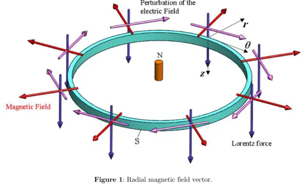
Consider a radial magnetic field vector H as shown in Figure 1. The resulting Lorentz force
(fz) and the perturbation of electric field vector
e
act along z and directions respectively.Now assume an annular circular plate with a uniform transverse load Po acting on its top
surface (see Fig. 2) is exposed to this magnetic field. As a result, the total transverse load
acting on the plate, along z direction, would be qz (qz=Po+ fz). This will induces a
Figure 1: Radial magnetic field vector.
Figure 2: Geometry, loading and coordinate system of the annular plate.
Assuming the magnetic permeability
(
z
)
of the plate is equal to the magneticpermeabil-ity of its surrounding, neglecting the displacement electric currents, the Maxwell’s electrody-namics equations for the plate may be written as (Wang and Dai, 2004);
j h
, ( ) ( )
H U curl H
U
( )( )
o
U
e z H
t , ( ) o h e z t (2)
where
j
is the surface density vector of the electric current,e
is the perturbation of theelectric field vector,
h
is the perturbation of the magnetic field vector and to is the time.On using cylindrical coordinates(r,,z), application of the magnetic field vectorH(Hr,0,0)
to Eqs. (1) and (2), results in;
) , 0 ,
(u w
U r , h(0,0,hz)
(3)
( )(0,0, r ( ))
w w
e z H
T r r
(4)
0, ( ),0
r w r w r H j r (5)
)
(
)
(
)
)(
(
2r
w
r
w
r
H
z
H
j
z
f
z r
(6))
(
r
w
r
w
H
h
z r
(7)
To deduce the equilibrium equations, it is assumed that the plate properties are distrib-uted along the thickness according to equations (8) - (10).
m t z z g ) 2 1 ( )
( (8)
2 1 (1 ( ))
) ( )
(z g z E g z E
E (9)
2 1 (1 ( ))
) ( )
(
z g z g z (10)Here, m is the volume fraction function power, t is the plate thickness which is assumed
to be uniform andE1,E2,
1and
2are the elastic moduli and magnetic permeabilitycoeffi-cients of phases 1 and 2 of the FG material, respectively (see Table 1, Ghorbanpour Arani et
al. 2010). Moreover, the Poisson’s ratio
of the plate is considered to be constant.FGM plate properties
Phase Material E (GPa) µ (H / m) ν
1 ( Ceramic ) Zirconia 151 2.63225901 E-6 0.3
2 ( Metal ) Aluminum 70 1.256665081 E-6 0.3
Table 1: Mechanical properties of the individual constituents used for the
In axisymmetric problems, deflection w, stresses and strains are independent of the
cir-cumferential direction and hence, their derivatives with respect to
are equal to zero.Con-sequently, in the present study, due to axisymmetric loading, deflection w becomes only a
function of r and one may write;
dr r dw z r u z r
ur( , ) r0( ) ( ) (11a)
0 ) , (r z
u (11b)
) ( ) ,
(r z w r
w (11c)
Additionally:
2 2 0 ( )
dr r w d z dr du r
ur r
r
(12a) dr r dw r z r u u r r
ur 1 r ( )
0 (12b) 0
r z
z
(12c)where u0 is the displacement of the middle surface of the FGM plate. Using Hooke's law, the
radial and circumferential stresses are;
] [
1
2
r r E (13a) ] [1 2 r
E
(13b)Expressing the total potential energy as U Vf , then the strain energy U and the
potential energy of the external forces
V
f are equal to;dr dz r a b t t r r
2 2 ] [ 2U (14a)
dr w q r a b z
2 ( )
f
V (14b)
Application of minimum total potential energy (0 ) to the plate, results in equation
(15).
0
rQ rq w drdr d Q r M M r dr d u N N r dr d a b z r r r r
In Eq. (15), Qr and qz(qz=Po+fz) are the shear force resultant and transverse load, Ni
and, Mi
ir,
, are the resultant forces and moments, and
is the small transversenor-mal rotation about axis, respectively. Using equation (15), the equilibrium equations may
be written as follow:
0:
rN N
dr d
ur r (16a)
0: rMr M rQr
dr d
(16b)
0: rQr rqz
dr d w
(16c)
Simplifying Eqs. (16), one may write;
0
N N dr dN r r r (17a) 0 ) ( 1 2 2 2
q r
dr dM r dr dM r dr M d z r r (17b) where
/2
2 / t t r r dz N N (18a)
/2 2 / t t r r dz z M M (18b)
On using Eq. (12), Eq. (13) may be written as;
)] ) ( ) ( ( [ 1 ) ( 2 2 0 0 2 dr r dw r dr r w d z r u dr du z
E r r
r (19a) )] ) ( ) ( 1 ( [ 1 ) ( 2 2 0 0 2 dr r w d dr r dw r z dr du r u z
E r r
(19b)
Therefore;
0 2
2 11 12 11 12
0
12 11 12 11
( )
ˆ ˆ ˆ ˆ
ˆ ˆ ˆ ˆ 1 ( )
r r
r
du d w r
N A A dr B B dr
N A A u B B dw r
r dr r (20a) 0 2 2 11 12 11 12
0
12 11 12 11
( )
ˆ ˆ
ˆ ˆ
ˆ ˆ ˆ ˆ 1 ( )
r r
r
du d w r
M B B dr C C dr
M B B u C C dw r
where;
/2
2 11 11 11 2
/2
1
ˆ ˆ ˆ
( , , ) ( )( 1 , , )
1
t
t
A B C E z z z dz
(21a)/2
2
12 12 12 2
/2
ˆ ˆ ˆ
( , , ) ( )( 1 , , )
1 t
t
A B C E z z z dz
(21b)Based on Eqs. (17a) and (20a), one may write;
2 0 0 3 2 0 11
2 2 3 2 2
11
ˆ
( ) 1 ( ) 1 ( ) ( ) 1 ( ) 1 ( ) 0
ˆ
r r
r
d u r du r B d w r d w r dw r
u r
r dr r dr
dr r A dr dr r
(22)
On using Eqs. (17b) and (20b) and substitutingPo fzfor qz(r), one can obtain:
2
4 3 2
2
11 11 11
11 4 3 2 2 3 2 3 0 2 0 0
0 11 11 11 11
2 3 2 2 3
ˆ ˆ ˆ
2 ( )
( ) ( ) ( ) ( )
ˆ ( )
ˆ ˆ ˆ
( ) ( ) ˆ ( ) 2 ( ) ( ) (
r r
r r r r
r
C C C z H
d w r d w r d w r dw r
C z H
r r dr
dr dr r dr r
z H d u r B d u r B du r B
w r B u r
r dr
r dr dr r r
)p0
(23)
To solve the above equilibrium equations, four types of boundary conditions are consid-ered as follow;
1.Clamped-Clamped (C-C) supports; Here, the outer and inner edges of the plate are
clamped. In this case, the boundary conditions are;
0 ) ( , 0 ) ( , 0 ) ( , 0 ) ( dr a dw a w dr b dw b w
2.Simply supported-Clamped (SS-C); Here, the outer edge of the plate is clamped while
the inner edge is simply supported. In this case, the boundary conditions are;
( )
( ) 0 r( ) 0 , ( ) 0 0
dw a
w b , M b w a ,
dr
3.Free-Clamped (F-C); Here, the outer edge of the plate is clamped while the inner edge
is free. In this case, the boundary conditions are;
0 ) ( , 0 ) ( , 0 ) ( , 0 ) ( dr a dw a w b M b
Nr r
4.Simply supported-simply supported (SS-SS): Base on this type of boundary condition,
the outer and inner edges of the plate are simply supported. In this case, the boundary conditions are;
( ) 0 r( ) 0 , ( ) 0 r( ) 0
w b , M b w a , M a
3 GENERALIZED DIFFERENTIAL QUADRATURE (GDQ)
GDQ is a numerical method that approximates the derivative of a function with respect to a variable as the sum of weighted linear function values at all domain points. This may be written as; n i r w C dr r w d j n j k ij k i k ,..., 2 ,1 ) ( ) ( 1
(24)where n is the number of grid points in r direction. In this work, for interval b ≤r≤a,
Che-byshev polynomials are used to identify the grid points. These point are defined by Eq. (25).
1 1 cos ( 1)
2 1
i
i
r b a b
n
(25)
Additionally, the Lagrange interpolating polynomials are used for the test functions as:
) ( ) ( ) ( )
( (1)
i i i r M r r r M r g (26) where;
n j j r r r M 1 ) ( ) ( ,
n i j j j ii r r
r M , 1 ) 1 ( ( ) ( ) (27) therefore; 1
1 ijk
:
2,3,...,
1
,
1,2,...,
k k
ij ii ij
i
C
C
k C
C
for i
j
k
n
and i j
n
r
r
(28)and;
1,
: ,
1,2,...,
n
k k
ii ij
j j i
C
C
for i
j
i j
n
(29)In Eqs. (28) and (29), the terms Cij and Cii are defined as;
n j i j i for r M r r r M C j j i i
ij , , ,12,...,
) ( ) ( ) ( ) 1 ( ) 1 ( (30)
n
j
i
j
i
for
C
C
n i j j ijii
,
,
,1
2
,...,
, 1
(31)2 0
2 0 11 3
2 2
1 11 1
ˆ
0
ˆ
1,2,...,
n n
ij r i ij ij
ij r j ij j
j i i j i i
C
u
B
C
C
C
u
C
w
r
r
A
r
r
for i
n
(32)3 2 2
4 2
11 2 3
1 11 11
2 2
3 0
11 0
2 2 3
1
2
1
( )
1
( )
ˆ
ˆ
ˆ
( )
ˆ
2
1
1,2,..., ,
1,2,...,
n
ij q r q r
ij ij ij j
j i i i i
n
q r ij ij
i ij r j
j
i i i i
C
z H
z H
C
C
C
C
w
r
r
C
r
r C
z H
C
C
w
B
C
u
P
r
r
r
r
for i
n
q
nn
(33)For simplicity, we define each term in Eq. (32) as a separate parameter defined in Eqs. (34)- (38).
0 1 1 11 12 00
0
r rn nu
w
K
K
u
w
(34)
211
:
ij,
1,2,...,
ij n n
i
C
if i
j
K
C
for
i j
n
r
(35)
211 2
1
:
ij,
1,2,...,
ij n n
i i
C
if i
j
K
C
for
i j
n
r
r
(36)
11 3 212 2
11
ˆ
,
1,2,...,
ˆ
ij ij ijn n
i i
C
C
B
K
C
for
i j
n
r
r
A
(37)
F
1
0
(38)Similarly, the terms in Eq. (33) are defined in Eqs. (39)- (44).
0 1 1 21 22 00
0
r rn nu
w
K
K
u
w
(39)
3 221 11 2
2
ˆ
:
ij ij,
1,2,...,
ij n n
i i
C
C
if i
j
K
B
C
for
i j
n
r
r
3 221 11 2 3
2
1
ˆ
:
ij ij,
1,2,...,
ij n n
i i i
C
C
if i
j
K
B
C
for
i j
n
r
r
r
(41)
3 2
4 2
2
11
22 11 2
3
11
2
1
( )
ˆ
ˆ
:
( )
1
ˆ
,
1,2,..., ,
1,2,...,
ij q r
ij ij i i n n q r ij i i
C
z H
C
C
r
r
C
if i
j
K
C
z H
C
r
r C
for
i j
n
q
nn
(42)
3 2 4 2 2 1122 11 2 2
3 2
11 11
2
1
( )
ˆ
ˆ
:
( )
( )
1
ˆ
ˆ
,
1,2,..., ,
1,2,...,
ij q r
ij ij
i i
n n
q r q r
ij
i i i
C
z H
C
C
r
r
C
if i
j
K
C
z H
z H
C
r
r C
r C
for
i j
n
q
nn
(43)
F
1
P
0 (44)According to Eqs. (32) to (44), equilibrium Eqs. (32) and (33) may be written in a matrix form as;
0 11 12 021 22 2 2 2 1 2 1
0
r
n
n n n
u
K
K
P
K
K
w
(45)Here, n and nn are the total number of grid points in r and z directions respectvely. In
Eqs. (45), the determinant of matrix [K] is equal to zero. Application of the previously
de-scribed boundary conditions to Eq. (45) results in values of wi (i = 1, n) and ui (i = 1, n).
Using these values, one can calculate the radial and tangential stresses in each case..
4 NUMERICAL RESULTS AND DISCUSSION
To investigate the effect of plate geometric parameters on the induced displacements and stresses, it is assumed that the annular FGM plate is experiencing a uniform mechanical load
4 0 10 ( 2)
N P
m
and a magnetic field of
m A
Hr3106 . The bottom and top surfaces of the
2 2
r r
o
t P a
, 22
o
t P a
,
o z z
P f
f , z
z r
h h
H
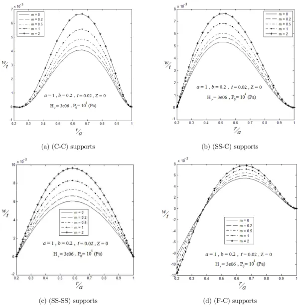
Figures 3 shows the variation in midplane deflection in terms of r
a , based on four
differ-ent types of boundary conditions given in section 2. In all cases, the transverse load qz is the
sum of mechanical and magnetic loads. According to this figure, for all values of m, the plate
deflection is maximum at r 0.66
a for case (a), while for case (b), it occurs at 0.52
r
a . For
cases (c), and (d), this value occurs at r 0.60
a , and free inner edge of the plate, respectively.
(a) (C-C) supports (b) (SS-C) supports
(c) (SS-SS) supports (d) (F-C) supports
Figure 3: The effect of parameter m on transverse deflection of the plate for
three different support conditions.
As expected, the (C-C) condition experiences the least deflection among all cases. In all
cases, a pure ceramic plate with m = 0, experiences the least deflection compared to other
values of m. This is due to an increase in flexural rigidity of the plate which is caused by a
decrease in m.
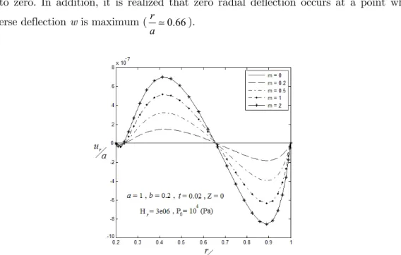
To investigate the effect of parameter m on radial deflection, a typical (C-C) plate with
similar loads and dimensions was selected. According to the results shown in Fig. 4, any
in-crease in power ratio m has a similar effect on midplane radial displacement. According to
these results, for a homogeneous plate with m = 0, the radial displacement of the midplane is
equal to zero. This is due to symmetry in mechanical properties of the plate which makes B11
equal to zero. In addition, it is realized that zero radial deflection occurs at a point where
transverse deflection w is maximum (r 0.66
a ).
Figure 4: The effect of parameter m on the midplane radial displacements, (C-C) supports.
Further examination of the results revealed that as long as a
b ratio remained equal to 5,
zero radial displacement occurred atr 0.66
a , regardless of the value for m (see Fig. 5).
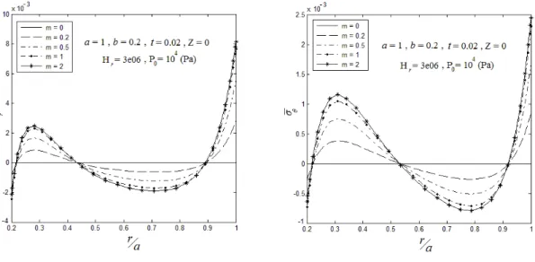
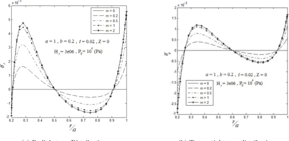
Figures 6-9 show the variation in radial and tangential stresses in midplane due to a
combination of transverse load Po and a radial magnetic field H. The plate dimensions for
different values of m are given in each figure. According to these figures, for all types of
boundary conditions discussed before, higher values of m (0 m 2) result in higher
abso-lute magnitude of both stress components. For m = 0 (a homogeneous plate withB110),
Figure 5: The effect of variation in plate dimensions on radial displacement, (C-C) supports.
(a) Radial stress distribution (b) Tangential stress distribution
Figure 6: The effect of parameter m on the mid-plane radial stresses based on (C-C) supports.
(a) Radial stress Distribution (b) Tangential stress distribution
Figure 7: The effect of parameter m on the mid-plane radial stresses based on (SS-C) supports.
(a) Radial stress distribution (b) Tangential stress distribution
Figure 8: The effect of parameter m on the mid-plane radial stress based on (SS-SS) supports.
The effect of magnetic field variation on displacement and stress components are shown in Figs. 10-13, for a typical plate with clamped supports. These results are based on the value
of m = 1. Although not shown, similar behaviors were observed for other values of m.
According to Fig. 10, exposure of the plate to a radial magnetic field has a substantial
ef-fect on its deflection. Any increase in magnetic field H causes a decrease in plate deflection in
presence of a transverse load Po. The location of maximum displacement seems to barely
(a) Radial stress distribution (b) Tangential stress distribution
Figure 9: The effect of parameter m on the midplane radial stresses based on (F-C) supports.
Figure 10: The effect of radial magnetic field variation H on plate transverse deflection w, (C-C) supports.
Similar effect was observed for radial deflection ur
a , in presence and absence of the
mag-netic field H (see Fig. 11). In either case, the magnitude of the transverse mechanical load is
Po. These results are extracted for m = 1. According to this figure, the presence of the radial
magnetic field shifts the location of zero radial displacement
u
r from r 0.57a to a 0.66 r
,
while substantially decreasing its extrema.
Figures 12 and 13 show the additional effect of magnetic field H on radial and tangential
vector substantially affects the location and values of both stresses at the inner and outer edges of the plate, as well as other locations. Additionally, any change from positive to nega-tive stresses in both directions seems to be highly affected by the presence of magnetic field.
Figure 11: The effect of radial magnetic field variation H on plate radial deflection, (C-C) supports.
Figure 13: The effect of radial magnetic field variation H on plate tangential stress, (C-C) supports.
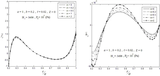
Figures 14-17 show the variation in Lorentz force and the induction magnetic field inten-sity along the plate radius, for the four types of boundary conditions discussed before. The
results are given for the plate midplane. Unlike the Lorentz force, distribution of
h
z along theplate radius appears to be a function of m. Higher values of m result in higher values of
h
z.(a) Lorentz force distribution (b) Induction magnetic field intensity distribution
Figure 14: The effect of variation in power m on (a) Lorentz force fz and
(a) Lorentz force distribution (b) Induction magnetic field intensity distribution
Figure 15: The effect of variation in power m on (a) Lorentz force fz and
(b) induction magnetic field intensity for (SS-C) supports.
(a) Lorentz force distribution (b) Induction magnetic field intensity distribution
Figure 16: The effect of variation in power m on (a) Lorentz force fz and
(b) induction magnetic field intensity for (SS-SS) supports.
(a) Lorentz force distribution (b) Induction magnetic field intensity distribution
Figure 17: The effect of variation in power m on (a) Lorentz force fz and
(b) induction magnetic field intensity for (F-C) supports.
Figures 18-21 show the effect of variation in plate geometry on the resulting stress and displacement components for a plate with a typical (C-C) boundary conditions. Here, the
three geometric parameters a, b and t are changed in the same proportion. Other parameters
are kept the same as before. According to Figs. 18 and 19, location of maximum w and zero
radial displacement barely depends on the plate dimensions.
Additionally, reducing the plate dimensions will lower the magnitude of displacement components, and hence relevant stresses are reduced, as shown in Figs. 20 and 21. This is due to plate stiffening as a result of lower dimensions and lower plate’s inner radius.
Figure 19: The effect of variation in plate dimensions on radial displacement, (C-C) supports.
Figure 21: The effect of variation in plate dimensions on tangential stress distribution , (C-C) supports.
The effect plate dimensions on Lorentz force and the induction magnetic field intensity are shown in Figs. 22 and 23, for a typical plate with (C-C) supports. According to Fig. 22, in
contrast with
h
z, the Lorentz force distribution along the plate radius does not seem tode-pend much on the plate dimensions. Figure 23 indicates that any change in the plate
dimen-sions barely affects the location of zero value for
h
z.Figure 23: The effect of plate dimensions on the induction magnetic field intensity distribution, (C-C) supports.
Figure 24 shows the transverse displacement of different points across the plate thickness
at r 0.66
a (location of maximum transverse deflection). The results are plotted for different
values of m in Fig. 24(a) and different values of Hr in Fig. 24(b). The applied loads and
boundary conditions, as well as the plate dimensions are as shown. According to Fig. 24(a),
for an isotropic plate with m=0, all points across the plate thickness have the same
deflec-tion. For higher values of m, the transverse deflection becomes more gradual across the plate
thickness. According to Fig. 24(b), any variation in Hr does not seem to highly affect the
transverse deflection across the plate thickness.
Figures 25 and 26 show the variation in Lorentz force and the induction of magnetic field
intensity across the plate thickness. According to these Figures, for m=0,
f
zandh
z arecon-stant along the plate thickness. For other values of m, the distribution of Lorentz force and
the induced magnetic field intensity across the plate thickness appear to highly depend on m.
The results on these figures are based on 0.66
a
r (location of maximum transverse
deflec-tion). According to figure 25, the magnitude of
h
z is the highest on the top surface of the(a) Variation in m (b) variation in Hr
Figure 24: The effect of parameter m and Hr on transverse deflection of the
plate along z direction, (C-C) supports.
Figure 25: The effect of power m on distribution of the induction magnetic
Figure 26: The effect of power m on Lorentz force distribution along the plate thickness, (C-C) supports.
Variations in radial and tangential stress components along the plate thickness are shown in Figs. 27 and 28, respectively. The results are for a typical plate with clamped supports. It
is assumed that m = 1 and 0.66
a
r (location of maximum transverse deflection). For small
values of Hr both stress components seem to change almost linearly across the plate thickness.
The maximum values of both stress components appear to be at top surface of the plate.
Figure 27: The effect of radial magnetic field on radial stress component
Figure 28: The effect of radial magnetic field on tangential stress component across the plate thickness, (C-C) supports.
It is worth to mention that based on the values given in Figs. 12-13 and 27-28, for all
values of Hr, zero radial and tangential stresses occur both in radial and transverse directions.
The locations of zero stress components across the plate thickness appear to be on a surface
which is slightly above the z =0 plane.
5 CONCLUSIONS
In this work, the radial and transverse displacements, as well as the radial and circumferen-tial stress components in an annular FGM plate subjected to a combination of transverse
load Po and Lorentz force fz, were calculated based on four types of boundary conditions. The
elastic modulus of the plate as well as the magnetic permeability coefficient across the plate thickness were assumed to vary according to the volume distribution function, while the Pois-son’s ratio was taken to be constant. Classical plate theory was applied to analyze the prob-lem. The deduced equilibrium equations were solved using generalized differential quadrature
method. According to the results, the effect of additional load fz induced by the radial
mag-netic field H seems to be substantial on plate radial and transverse deflections. Additionally,
in presence of a transverse load Po, application of a radial magnetic field to the plate top
surface, completely changes the state of tangential and radial stresses along its radius, resulting in positive and negative stresses in these two directions. The effect of additional
transverse load fz induced by the magnetic field vector Hon both stress components across
the plate thickness seems to be more on bottom surface (pure metal). Moreover, the
magnitude of the Lorentz force and the induced magnetic field intensity
h
z across the platemagnetic field Hr to a plate which is already loaded by a transverse load Po reduces the plate
displacement and stress components, and hence, resulting in a higher factor of safety in the plate.
References
Bayat, M., Rahimi, M., Saleem, M., Mohazzab, A.H., Wudtke, I., Talebi, H., (2014). One-dimensional analy-sis for magneto-thermo-mechanical response in a functionally graded annular variable-thickness rotating disk. Applied Mathematical Modelling 38:4625–4639.
Behravan Rad, A., Shariyat, M., (2015). Three-dimensional magneto-elastic analysis of asymmetric variable thickness porous FGM circular plates with non-uniform tractions and Kerr elastic foundations. Composite Structures, 125: 558–574.
Chi, S.H., Chung, Y.L., (2006). Mechanical behavior of functionally graded material plates under transverse load—Part I: Analysis. International Journal of Solids and Structures, 43: 3657–3674.
Ghorbanpour Arani, A., Loghman, A., Shajari, A. R., Amir, S. (2010). Semi-analytical solution of magneto-thermo-elastic stresses for functionally graded variable thickness rotating disks. Journal of Mechanical Science and Technology 24 (10): 2107-2117
Lal, R. and Saini, R. (2015). Buckling and Vibration of Functionally Graded Non-uniform Circular Plates Resting on Winkler Foundation. Latin American Journal of Solids and Structures 12(12): 2231-2258.
Lal, R. and Saini, R. (2015). On the use of GDQ for vibration characteristic of non-homogeneous orthotropic rectangular plates of bilinearly varying thickness. Acta Mechanica, 226: 1605–1620.
Ma, L.S., Wang, T.J., (2003). Nonlinear bending and post-buckling of a functionally graded circular plate under mechanical and thermal loadings. International Journal of Solids and Structures 40: 3311–3330.
Najafizadeh, M.M., Heydari, H.R., (2004). Thermal buckling of functionally graded circular plates based on higher order shear deformation plate theory. European Journal of Mechanics A/Solids 23: 1085–1100.
Praveen, G.N., Reddy, J.N., (1998). Non-linear transient thermoelastic analysis of functionally graded Ceram-ic-Metal plates. International Journal of Solids and Structures 35: 4457–4476.
Reddy, J.N., (2000). Analysis of functionally graded plates. Int. J. Numer. Methods Eng 47: 663-684.
Reddy, J.N., Wang, C.M., Kitipornchai, S., (1999). Axisymmetric bending of functionally graded circular and annular plates. European Journal of Mechanics A/Solids 18: 185-199.
Saidi, A.R., Rasouli, A., Sahraee, S., (2009). Axisymmetric bending and buckling analysis of thick functional-ly graded circular plates using unconstrained third-order shear deformation plate theory. Composite Struc-tures 89: 110-119.
Wang, X., Dai, H.L. (2004). Magneto thermodynamic stress and perturbation of magnetic field vector in an orthotropic thermoelastic cylinder. International Journal of Engineering Science 42: 539–556.