www.atmos-chem-phys.net/14/5807/2014/ doi:10.5194/acp-14-5807-2014
© Author(s) 2014. CC Attribution 3.0 License.
Estimating Asian terrestrial carbon fluxes from CONTRAIL
aircraft and surface CO
2
observations for the period 2006–2010
H. F. Zhang1,2, B. Z. Chen1, I. T. van der Laan-Luijkx3, T. Machida4, H. Matsueda5, Y. Sawa5, Y. Fukuyama6, R. Langenfelds7, M. van der Schoot7, G. Xu1,2, J. W. Yan1,2, M. L. Cheng1,2, L. X. Zhou8, P. P. Tans9, and W. Peters3,10 1State Key Laboratory of Resources and Environment Information System, Institute of Geographic Sciences and Natural
Resources Research, Chinese Academy of Sciences, Beijing 100101, China
2University of Chinese Academy of Sciences, Beijing 100049, China
3Department of Meteorology and Air Quality (MAQ), Wageningen University, Droevendaalsesteeg 3a, 6700 PB,
Wageningen, the Netherlands
4Center for Global Environmental Research, National Institute for Environmental Studies, Tsukuba, Japan 5Geochemical Research Department, Meteorological Research Institute, Tsukuba, Japan
6Atmospheric Environment Division, Global Environment and Marine Department, Japan Meteorological Agency, Japan 7Centre for Australian Weather and Climate Research/CSIRO Marine and Atmospheric Research, Aspendale, Victoria,
Australia
8Key Laboratory for Atmospheric Chemistry of China Meteorological Administration, Research Institute of Atmospheric
Composition of Chinese Academy of Meteorological Sciences, Beijing 100081, China
9Earth System Research Laboratory, National Oceanographic and Atmospheric Administration, Boulder,
Colorado 80305, USA
10Centre for Isotope Research, Groningen, the Netherlands
Correspondence to:B. Z. Chen ([email protected]) and W. Peters ([email protected]) Received: 9 October 2013 – Published in Atmos. Chem. Phys. Discuss.: 24 October 2013
Revised: 16 April 2014 – Accepted: 25 April 2014 – Published: 11 June 2014
Abstract. Current estimates of the terrestrial carbon fluxes in Asia show large uncertainties particularly in the boreal and mid-latitudes and in China. In this paper, we present an updated carbon flux estimate for Asia (“Asia” refers to lands as far west as the Urals and is divided into bo-real Eurasia, temperate Eurasia and tropical Asia based on TransCom regions) by introducing aircraft CO2
measure-ments from the CONTRAIL (Comprehensive Observation Network for Trace gases by Airline) program into an inver-sion modeling system based on the CarbonTracker frame-work. We estimated the averaged annual total Asian terres-trial land CO2sink was about−1.56 Pg C yr−1over the
pe-riod 2006–2010, which offsets about one-third of the fossil fuel emission from Asia (+4.15 Pg C yr−1). The uncertainty
of the terrestrial uptake estimate was derived from a set of sensitivity tests and ranged from−1.07 to−1.80 Pg C yr−1,
comparable to the formal Gaussian error of±1.18 Pg C yr−1
(1-sigma). The largest sink was found in forests,
predom-inantly in coniferous forests (−0.64±0.70 Pg C yr−1) and mixed forests (−0.14±0.27 Pg C yr−1); and the second and third large carbon sinks were found in grass/shrub lands and croplands, accounting for −0.44±0.48 Pg C yr−1 and −0.20±0.48 Pg C yr−1, respectively. The carbon fluxes per
ecosystem type have large a priori Gaussian uncertainties, and the reduction of uncertainty based on assimilation of sparse observations over Asia is modest (8.7–25.5 %) for most individual ecosystems. The ecosystem flux adjust-ments follow the detailed a priori spatial patterns by de-sign, which further increases the reliance on the a priori biosphere exchange model. The peak-to-peak amplitude of inter-annual variability (IAV) was 0.57 Pg C yr−1 ranging
from−1.71 Pg C yr−1 to−2.28 Pg C yr−1. The IAV
analy-sis reveals that the Asian CO2sink was sensitive to climate
variations, with the lowest uptake in 2010 concurrent with a summer flood and autumn drought and the largest CO2
5808 H. F. Zhang et al.: Estimating Asian terrestrial carbon fluxes
precipitation conditions. We also found the inclusion of the CONTRAIL data in the inversion modeling system reduced the uncertainty by 11 % over the whole Asian region, with a large reduction in the southeast of boreal Eurasia, southeast of temperate Eurasia and most tropical Asian areas.
1 Introduction
The concentration of carbon dioxide (CO2)has been
increas-ing steadily in the atmosphere since the industrial revolu-tion, which is considered very likely to be responsible for the largest contribution of the climate warming (Huber and Knutti, 2011; Peters et al., 2011). Knowledge of the terres-trial carbon sources and sinks is critically important for un-derstanding and projecting the future atmospheric CO2
lev-els and climate change. The global terrestrial ecosystems ab-sorbed about 1–3 Pg carbon every year during the 2000s, with obvious interannual variations, offsetting 10–40 % of the anthropogenic emissions (Le Quéré et al., 2009; Maki et al., 2010; Saeki et al., 2013). However, estimates of the ter-restrial carbon balance vary considerably when considering continental scales and smaller, as well as when estimating the CO2seasonal and inter-annual variability (Houghton, 2007;
Peylin et al., 2013).
Asia, as one of the biggest Northern Hemisphere terres-trial carbon sinks, has a significant impact on the global car-bon budget (Jiang et al., 2013; Patra et al., 2012; Piao et al., 2009, 2012; Peylin et al., 2013; Yu et al., 2013). It is es-timated that Asian ecosystems contribute over 50 % of the global net terrestrial ecosystem exchange (Maksyutov et al., 2003) and their future balance is thought to be a great source of uncertainty in the global carbon budget (Ichii et al., 2013; Oikawa and Ito, 2001). Even though the importance of the Asian ecosystems is increasingly recognized and many ef-forts have been carried out to estimate the Asian terrestrial carbon sources and sinks, they still remain poorly quantified (Ito, 2008; Patra et al., 2012, 2013; Piao et al., 2011). One reason is that a steep rise of fossil fuel emissions in most Asian countries has imposed large influences on the Asian CO2balance and leads to an increased variability of the
re-gional carbon cycle (Francey et al., 2013; Le Quere et al., 2009; Patra et al., 2011, 2013; Raupach et al., 2007). In ad-dition, rapid land-use change and climate change have likely increased the variability in the Asian terrestrial carbon bal-ance (Cao et al., 2003; Patra et al., 2011; Yu et al., 2013). This makes it challenging to accurately estimate CO2fluxes
of the Asia ecosystems.
Currently two approaches are commonly used to esti-mate CO2 fluxes at regional to global scales: the so-called
“bottom-up” and “top-down” methods. The bottom-up ap-proach is based on local data or field measurements to retrieve the carbon fluxes, including direct measurements (Chen et al., 2012; Clark et al., 2001; Fang et al., 2001;
Mi-zoguchi et al., 2009; Takahashi et al., 1999) and ecosystem modeling (Chen et al., 2007; Fan et al., 2012; Randall et al., 1996; Randerson et al., 1997; Sellers et al., 1986, 1996). The top-down method uses atmospheric mole fraction data to derive the CO2sink/source information. As one of the
im-portant “top-down” approaches, atmospheric inverse model-ing has been well developed and widely applied (Baker et al., 2006; Chevallier and O’Dell, 2013; Deng et al., 2007; Gurney et al., 2003; Gurney et al., 2004), and has shown to be particularly successful in estimating regional carbon flux for regions rich in atmospheric CO2 observations like
North America and Europe (Broquet et al., 2013; Deng et al., 2007; Peters et al., 2007, 2010; Peylin et al., 2005, 2013; Rivier et al., 2011, 2010). However, estimating Asian CO2
surface fluxes with inverse modeling remains challenging, and the inverted Asian CO2 fluxes still exhibit a large
un-certainty partly because of a lack of surface CO2
observa-tions. For example, in the TransCom3 annual mean con-trol inversion, Gurney et al. (2003) used a set of 17 mod-els to estimate the carbon fluxes and obtained different re-sults for the Asian biospheric CO2budget, ranging from a
large CO2source of+1.00±0.61 Pg C yr−1to a large sink of −1.50±0.67 Pg C yr−1for the year 1992–1996. In the
REC-CAP (REgional Carbon Cycle Assessment and Processes) project, Piao et al. (2012) presented the carbon balance of terrestrial ecosystems in East Asia from eight inversions dur-ing the period 1990–2009. The results from these eight in-version models also show disagreement. Six models esti-mate a net CO2uptake with the highest net carbon sink of −0.997 Pg C yr−1, while two models show a net CO
2source
with the largest net carbon emission of+0.416 Pg C yr−1in
East Asia. The important role of the sparse observational net-work was demonstrated by Maki et al. (2010), who reported a large Asian land sink of−1.17±0.50 Pg C yr−1or much
smaller sink of−0.65±0.49 Pg C yr−1over the Asian region
depending on which set of observations was included in the same inversion system. This situation suggests that a more accurate estimate of the surface CO2flux is urgently required
in Asia, and the ability to base it on as much observational data as possible is key.
To expand the number of CO2 observations, the aircraft
project CONTRAIL has measured CO2 mole fractions
on-board passenger flights since 2005, and has produced a large coverage of in situ CO2data ranging over various latitudes,
longitudes, and altitudes (Machida et al., 2008; Matsueda et al., 2008). CONTRAIL observations have also already suc-cessfully been used to constrain surface flux estimates (Niwa et al., 2011, 2012; Patra et al., 2011). Patra et al. (2011) reported the added value of CONTRAIL data to inform on tropical Asian carbon fluxes, as their signals are transported rapidly to the free troposphere over the west Pacific.
In this study, we also used the CONTRAIL CO2
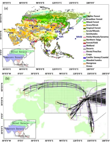
Figure 1. (a)Map of the Asian surface observation sites, along with the map of the ecoregion types from Olson et al. (1985) with 19 land cover classes as used in this study. These Asian surface obser-vation data download from the NOAA-ESRL (e.g., Mt. Waliguan, China (WLG), Bukit Kototabang, Indonesia (BKT), Sede Boker, Is-rael (WIS), Sary Taukum, Kazakhstan (KZD), Plateau Assy, Kaza-khstan (KZM), Tae-ahn Peninsula,South Korea (TAP), Ulaan Uul, Mongolia (UUM), Cape Rama, India (CRI)) and WDCGG network (e.g., Lulin, Taiwan (LLN), Shangdianzi, China (SDZ), Minamitor-ishima, Japan (MNM), Ryori, Japan (RYO), Yonagunijima, Japan (YON), Gosan, South Korea (GSN));(b)CONTRAIL CO2
obser-vations map, along with 42 horizontal regions. The red rectangles represent the nine regions covering the ascending and descending data (included four vertical bins at 575–625, 475–525, 375–425, 225–275 hPa) over airports, and the blue rectangles indicate the other 33 regions covering the cruise data (included one bin at 225– 275 hPa). The big black rectangle indicates a zoom region over Asia (1◦×1◦) based on global grid (3◦×2◦). Note that “Asia” refers to lands as far west as the Urals in this study and it is further divided into boreal Eurasia, temperate Eurasia and tropical Asia based on TransCom regions (Gurney et al., 2002; Gurney et al., 2003). These divided regions are presented in the small inset in the bottom left corner (same as thereafter).
period 2006–2010. Our inversion model is the state-of-the-art CO2 data assimilation system CTDAS (CarbonTracker
Data Assimilation Shell, http://carbontracker.eu/ctdas/). Our work complements previous inverse modeling studies as it (1) presents the inverted CO2 results of Asian weekly net
ecosystem exchange not shown previously; (2) uses surface
observations not available in earlier top-down estimates; (3) assimilates the continuous CO2 observation from a number
of Asian continental sites for the first time; (4) includes extra free tropospheric CO2observations to further constrain the
estimate; (5) uses a two-way atmospheric transport model TM5 (Krol et al., 2005) with higher horizontal resolution than previous global CO2 data assimilation studies that
fo-cused on Asia (this study uses a 1◦×1◦grid over Asia while
globally a 2×3◦resolution, see Fig. 1b).
This paper is organized as follows. Methods and materi-als are described in Sect. 2, the inferred Asian land flux and its temporal-spatial variations are presented in Sect. 3. To examine the impact of CONTRAIL data on Asian flux es-timates, we also compared inverse results with and without CONTRAIL data during the period 2006–2010. In Sect. 4, we compare our inverted Asian surface fluxes with previous findings and discuss our uncertainty estimates and future di-rections. Note that “Asia” refers to lands as far west as the Urals, and it is further divided into boreal Eurasia, temperate Eurasia and tropical Asia based on TransCom regions (Gur-ney et al., 2002, 2003) (see small inset in the bottom left corner of Fig. 1).
2 Methods and data sets
2.1 The atmospheric inversion model (CTDAS)
The atmospheric inverse model CTDAS was developed by NOAA-ESRL (National Oceanic and Atmospheric Admin-istration’s Earth System Research Laboratory) and Wagenin-gen University, the Netherlands. Previous versions of the sys-tem have been applied successfully in North America and Europe (Masarie et al., 2011; Peters et al., 2007, 2010). CTDAS was designed to estimate net CO2 terrestrial and
oceanic surface fluxes by integrating atmospheric CO2
con-centration measurements, a global transport model, and a Bayesian synthesis technique that minimizes the difference between the simulated and observed CO2 concentrations.
The first step is the forecast of the atmospheric CO2
concen-trations using the transport model TM5 (Krol et al., 2005) with a global resolution of 3◦×2◦ and 1◦×1◦ over Asia
(Fig. 1b). The TM5 transport model is driven by meteorolog-ical data of the ERA-interim analysis of the European Centre for Medium-Range Weather Forecasts (ECMWF), and prop-agates four separate sets of bottom-up fluxes (details are pre-sented in Sect. 2.2). The forecasted four-dimensional (4-D) concentrations (x, y, z, t) are sampled at the location and time of the observed atmospheric CO2mole fractions, and
subse-quently compared. The difference between the observed and simulated CO2concentrations is minimized. This
5810 H. F. Zhang et al.: Estimating Asian terrestrial carbon fluxes
As described in Peters et al. (2007), four a priori and im-posed CO2fluxes integrate in CTDAS to instantaneous CO2
fluxesF (x,y,t) as follows:
F (x, y, t )=λrFbio(x, y, t )+λrFoce(x, y, t )
+Fff(x, y, t )+Ffire(x, y, t ), (1)
whereFbioandFoceare 3-hourly, 1◦×1◦a priori terrestrial
biosphere and ocean fluxes, respectively; Fff and Ffire are
monthly 1◦×1◦prescribed fossil fuel and fire emissions, and λris a set of weekly scaling factors, and each scaling factor is
associated with a particular region of the global domain that is divided into 11 land and 30 ocean regions according to climate zone and continent. Nineteen ecosystem types (Ol-son et al., 1985) (Fig. 1a) have been considered in each of the 11 global land areas (Gurney et al., 2002), dividing the globe into 239 regions (239=11 land×19 ecosystem types
+30 ocean regions). The actual region number assimilated
in this system is 156, after excluding 83 regions which are associated with a non-existing ecosystem (such as “snowy conifers” in Africa). The corresponding scaling factors have been estimated as the final product of CTDAS, and have been applied to obtain the terrestrial biosphere and ocean fluxes at the ecosystem and ocean basin scale by multiplying them with the a priori fluxes. The adjusted fluxes are then put into the transport model to produce an optimized 4-D CO2mole
fraction distribution.
2.2 A priori CO2flux data set
In CTDAS, four types of CO2surface fluxes are considered
as follows: (1) the a priori estimates of the oceanic CO2
ex-change are based on the air–sea CO2partial pressure
differ-ences from ocean inversions results (Jacobson et al., 2007). These air–sea partial pressure differences are combined with a gas transfer velocity computed from wind speeds in the atmospheric transport model to compute fluxes of carbon dioxide across the sea surface every 3 h; (2) the a priori ter-restrial biosphere CO2fluxes are from GFED2 (Global Fire
Emissions Database version 2), which is derived from the Carnegie–Ames Stanford Approach (CASA) biogeochemi-cal modeling system (Van der Werf et al., 2006). A monthly varying NEE flux (NEE=Re−GPP) was constructed from
the following two flux components: gross primary produc-tion (GPP) and ecosystem respiraproduc-tion (Re), and interpolated
to 3-hourly net land surface fluxes using a simple temper-ature Q10 relationship assuming a globalQ10 value of 1.5
for respiration, and a linear scaling of photosynthesis with solar radiation. (3) The imposed fossil fuel emission esti-mates from the global total fossil fuel emission of the CDIAC (Carbon Dioxide Information and Analysis Center) (Marland et al., 2003) were spatially and temporally interpolated fol-lowing the EDGAR (Emission Database for Global Atmo-spheric Research) database (Boden et al., 2011; Commis-sion, 2009; Olivier and Berdowski, 2001; Thoning et al., 1989); (4) the biomass-burning emissions are from GFED2,
which combines monthly burned area information observed from satellites (Giglio et al., 2006) with the CASA biogeo-chemical model. Fire emissions in GFED2 are available only up to 2008, so for 2009 and 2010 we use a climatology of monthly averages of the previous decade. Note that GFED3 (and now even GFED4) is available for quite a few years, and offers higher spatial resolutions in biomass-burning emis-sions that are attractive for model simulation. But it uses a different product for the satellite observed NDVI (Nor-malized Difference Vegetation Index) and FPAR (the Frac-tion of Photosynthetically Active RadiaFrac-tion) (MODIS (the MODerate resolution Imaging Spectroradiometer) instead of AVHRR (Advanced Very High Resolution Radiometer)) which causes a different seasonality in the biosphere fluxes which are calculated alongside the fire emissions in GFED, with a less realistic amplitude. Since this amplitude of the seasonal biosphere is important to us, we did not update to this new GFED3 product. We also tested the GFED4 data with SIBCASA (Simple Biosphere/Carnegie-Ames-Stanford Approach) to make a new data set of fire estimates but our analyses showed that the impact of using GFED4 versus GFED2 on estimated Asia fluxes is very weak.
2.3 Atmospheric CO2observations
In this study, two sets of atmospheric CO2 observation
data were assimilated as follows: (1) surface CO2
obser-vations distributed by NOAA-ESRL (http://www.esrl.noaa. gov/gmd/ccgg/obspack/, data version 1.0.2) and by the WD-CGG (World Data Centre for Greenhouse Gases, http://ds. data.jma.go.jp/gmd/wdcgg/) for the period 2006–2010 (the Asian surface site information is summarized in Fig. 1a and the global surface sites in Table S1 of the Supplement). Indi-vidual time series in this surface set were provided by many individual PIs (Principal Investigators) which we kindly ac-knowledge; (2) for the free tropospheric CO2observations,
we use the aircraft measurements from the CONTRAIL project for the period 2006–2010 (see Fig. 1b).
A summary of Asian surface sites used in this study is shown in Table 1 and Fig. 1a for reference. There are fourteen surface sites with over 7957 observations located in Asia, in-cluding ten surface flask stations and four surface continuous sites. The surface CO2mole fraction data used in this study
are all calibrated against the same CO2 standard
(WMO-X2007) (The World Meteorological Organization CO2mole
fraction scale for 2007). For most of the continuous sam-pling sites at the surface, we derived an averaged afternoon CO2 concentration (12:00–16:00, local time) for each day
from the time series, while at mountain-top sites we con-structed an average based on nighttime hours (00:00–04:00, local time) to reduce local influence and compare modeled with observed values only for well-mixed conditions.
We note that from the CONTRAIL program (Machida et al., 2008; Matsueda et al., 2008), stratospheric CO2 data
Table 1.Summary of the 14 Asian surface CO2observation sites assimilated between 1 January 2006 and 31 December 2010. The frequency
of continuous data is one per day (when available), while discrete surface data point is generally available once per week. MDM (model–data mismatch) is a value assigned to a given site that is meant to quantify our expected ability to simulate observations and used to calculate the innovationX2(Inn.X2)statistics.Ndenotes the number of observations used in CTDAS. Flagged observations refer to a model-minus-observation difference that exceeds 3 times the model–data mismatch, these model-minus-observations are therefore excluded from assimilation. The bias is the average from posterior residuals (assimilated values–measured values), while the modeled bias is the average from prior residuals (modeled values–measured values).
Site Name Lat, Lon, Elev. Lab N MDM Inn. Bias(modeled) (flagged) X2
Discrete samples in Asia:
1 WLG Mt. Waliguan, China 36.29◦N, 100.90◦E, 3810 m CMA/ESRL 254(19) 1.5 0.83 −0.10(−0.14) 2 BKT Bukit Kototabang, Indonesia 0.20◦S, 100.312◦E, 864 m ESRL 172(0) 7.5 0.73 5.53(5.51) 3 WIS Sede Boker, Israel 31.13◦N, 34.88◦E, 400 m ESRL 239(1) 2.5 0.62 −0.10(−0.15) 4 KZD Sary Taukum, Kazakhstan 44.45◦N, 77.57◦E, 412 m ESRL 167(6) 2.5 1.16 −0.08(0.50) 5 KZM Plateau Assy, Kazakhstan 43.25◦N, 77.88◦E, 2519 m ESRL 155(2) 2.5 0.96 0.50(0.63) 6 TAP Tae-ahn Peninsula, South Korea 36.73◦N, 126.13◦E, 20 m ESRL 181(3) 7.5 0.60 1.82(2.13) 7 UUM Ulaan Uul, Mongolia 44.45◦N, 111.10◦E, 914 m ESRL 231(5) 2.5 1.17 0.10(0.28) 8 CRI Cape Rama, India 15.08◦N, 73.83◦E, 60 m CSIRO 33(1) 3 1.40 −1.97(−2.11) 9 LLN Lulin, Taiwan 23.47◦N, 120.87◦E, 2862 m ESRL 220(20) 7.5 0.99 2.62(2.65) 10 SDZ Shangdianzi, China 40.39◦N, 117.07◦E, 287 m CMA/ESRL 60(15) 3 1.18 0.15(0.18) continuous samples in Asia:
11 MNM Minamitorishima, Japan 24.29◦N, 153.98◦E, 8 m JMA 1624(0) 3 0.76 0.15(0.16) 12 RYO Ryori, Japan 39.03◦N, 141.82◦E, 260 m JMA 1663(48) 3 0.90 0.46(0.69) 13 YON Yonagunijima, Japan 24.47◦N, 123.02◦E, 30 m JMA 1684(3) 3 0.78 1.53(1.67) 14 GSN Gosan, Republic of South Korea 33.15◦N, 126.12◦E, 72 m NIER 1274(109) 3 1.99 −1.01(−0.82)
observations had a seasonal phase shifting and its smaller amplitude was difficult to compare to the tropospheric mea-surements (Sawa et al., 2008). A summary of the CON-TRAIL aircraft measurements is presented in Table 2 and Fig. 1b. The CONTRAIL aircraft data are reported on the NIES (the National Institute for Environmental Studies) 09 CO2 scale, which are lower than the WMO−X2007 CO2
scale by 0.07 ppm at around 360 ppm and consistent in the range between 380 and 400 ppm (Machida et al., 2011). Thus the CONTRAIL CO2data sets are comparable to
sur-face data. We follow the method from Niwa et al. (2012) to divide the data into four vertical bins (575–625, 465– 525, 375–425, 225–275 hPa) from ascending and descend-ing profiles and one vertical bin (225–275 hPa) from level cruising. We also divide CONTRAIL data into 42 hori-zontal bins/regions (Fig. 1b), which amounts to a total of 65 bins. Before daily averaging the CONTRAIL measure-ments for each 65 regional/vertical bins, we pre-process the aircraft data to obtain free troposphere CO2 values by
fil-tering out the stratospheric CO2 data using a threshold of
potential vorticity (PV) > 2 PVU (Potential Vorticity Unit, 1 PVU=10−6m2s−1K kg−1), in which PV is calculated from TM5 (using ECMWF temperature, pressure and wind fields ) (Sawa et al., 2008). A total number of 10 467 CO2
aircraft observations over Asia have been used during the pe-riod from January 2006 to December 2010 in our inversion.
2.4 Sensitivity experiments and uncertainty estimation
Because the Gaussian uncertainties strongly de-pend on choices of prior errors in CTDAS, the formal covariance estimates for each week of optimization only reflect the random component of the inversion problem rather than a characterization of the true uncertainties of the estimated CO2 flux. As an alternative, we performed a set
of sensitivity experiments to obtain a more representative spread in the flux estimates and complement the formal Gaussian uncertainty estimates. We take different plausible alternative settings in CTDAS to design a more comprehen-sive sensitivity test, and use the minimum and maximum flux inferred in these experiments to present the range of the true flux. The following six inversions were performed to investigate the uncertainty span in this study:
Case 1: prior flux as in Sect. 2.2 + observations as in Sect. 2.3+TM5 transport model runs at global 3◦×2◦and
a 1◦×1◦nested grid over Asia. This is the base simulation
(quoted as surface–CONTRAIL) which is used to analyze the 5 year carbon balance in this study.
Case 2: same as Case 1, but excluding CONTRAIL ob-servations. We use these results (quoted as surface–only) to examine the impact of CONTRAIL data on Asian flux esti-mates by comparison with Case 1.
5812 H. F. Zhang et al.: Estimating Asian terrestrial carbon fluxes
Table 2.Summary of the Asian CONTRAIL CO2observation data
assimilated between 2006 and 2010. MDM (model–data mismatch) is a value assigned to a given site that is meant to quantify our ex-pected ability to simulate observations and used to calculate the in-novationX2(Inn.X2)statistics.N denotes the number available in CTDAS. Flagged observations mean a model-minus-observation difference that exceeds 3 times the model–data mismatch, these data are therefore excluded from assimilation. The bias is the average of the posterior residuals (assimilated values–measured values), while the modeled bias is the average of prior residuals (modeled values– measured values).
Pressure Level N(flagged) MDM Inn.X2 Bias(modeled) 575–625 hPa 0 2.00 0.00 0.00 475–525 hPa 2907(5) 2.00 0.35 0.05(0.08) 375–425 hPa 3035(3) 2.00 0.34 −0.05(−0.07) 225–275 hPa 4525(4) 2.00 0.34 0.04(0.05)
Different from fossil fuel data in Case 1, the data of Wang et al. (2012) calculated carbon emissions from energy con-sumption, transportation, household energy concon-sumption, commercial energy consumption, industrial processes and waste. And the seasonal variations between the two data sets are different. the fossil fuel emissions in Case 1 had the largest carbon emission in January and the smallest carbon source in July every year, while data of Wang et al. (2012) had the smallest fossil-fuel CO2 emissions in February or
March. This simulation is meant to partly address the im-pact of uncertainty in fossil fuel emissions over the region as suggested by Francey et al. (2013).
Case 4: like Case 1, but CTDAS runs based on 110 % of prior biosphere flux derived from CASA-GFED2;
Case 5: like Case 2, but the TM5 transport model is used at global 6◦×4◦without nested grids. This tests the impact of model resolution;
Case 6: like Case 2, but replacing the underlying land use map with MODIS data (Friedl et al., 2002) and keep-ing the number of ecoregions unchanged. The MODIS land use maps can be found in Fig. S1 in the Supplement.
The Cases 1 and 2 span the period 2006–2010 (the pe-riod 2004–2005 was discarded as spin-up), while the other sensitivity experiments were done from 2008 to 2010 only when the observational coverage was best. In general, these six sensitivity tests investigate most variations in the com-ponents of the assimilation framework. These variations are prior fluxes, observations available, the ecoregion map, the fossil fuel emissions, and transport. They also give alterna-tive choices for the main components of the system. The sen-sitivity results are summarized in Table 3 and further dis-cussed in the next section.
3 Results
We will from here on refer to carbon sinks with a negative sign, sources are positive, and will include the sign also when discussing anomalies (positive=less uptake or larger source,
negative=more uptake or smaller source). We describe the
results mainly over Asia (global flux estimates can be found in Table S2 in the Supplement), where we expected the CON-TRAIL data to provide the additional constraints. Note that the results of Case 1 are analyzed as the best assimilation for the period of 2006–2010 in this study.
3.1 CO2concentration simulations
First we checked the accuracy of the model simulation using the surface CO2concentration observations and CONTRAIL
aircraft CO2measurements. Figure 2a shows the comparison
of modeled (both prior and posterior) CO2concentration with
measurements at the discrete surface site of Mt. Waliguan (WLG, located at 36.29◦N, 100.90◦E). Note that the prior CO2concentrations here are not really based on a priori
fluxes only, as they are a forecast started from the CO2
mix-ing ratio field that contains all the already optimized fluxes (1, ...,n−1) that occurred before the current cycle of the data
assimilation system (n). So these prior mole fractions only contain five weeks of recent un-optimized fluxes and consti-tute our “first-guess” of atmospheric CO2for each site. For
the WLG site, the comparison of the surface CO2time series
shows that the modeled (both prior and posterior) CO2
con-centration is in general agreement with observed data dur-ing the period 2006–2010 (correlation coefficientR=0.87), although the modeled result still could not adequately re-produce all the observed CO2seasonal variations. The
pos-terior annual model–observation mismatch of this distri-bution is−0.10±1.25 ppm, with 0.07±1.50 ppm bias for
the summer period (June–July–August) and 0.02±0.80 ppm
bias for the winter period (December–January–February). The model–observation mismatch is a little larger in Case 2 without CONTRAIL data (model–observation mismatch:
−0.13±1.26 ppm), suggesting that the surface fluxes
de-rived with CONTRAIL agree with the surface CO2 mixing
ratios at WLG station. Over the full study period, the WLG modeled mole fractions exhibit good agreement with the ob-served CO2 time series and the changes in inferred mixing
ratios/flux are within the specified uncertainties in our inver-sion system, an important prerequisite for a good flux esti-mate.
We also checked the inversion performance in the free tro-posphere in addition to the surface CO2. Figure 2b, c and d
show the comparison between measured and modeled (both prior and posterior) mixing ratios in the free troposphere dur-ing the period from 2006–2010 in the region coverdur-ing 32– 40◦N, 136–144◦E for three vertical bins (475–525, 375– 425, 225–275 hPa). The observed vertical CO2patterns were
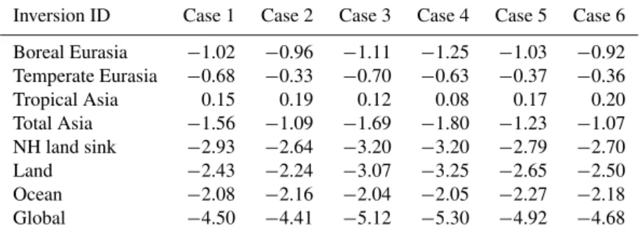
Table 3.Results of the sensitivity experiments conducted in this study (units of Pg C yr−1)∗.
Inversion ID Case 1 Case 2 Case 3 Case 4 Case 5 Case 6
Boreal Eurasia −1.02 −0.96 −1.11 −1.25 −1.03 −0.92 Temperate Eurasia −0.68 −0.33 −0.70 −0.63 −0.37 −0.36 Tropical Asia 0.15 0.19 0.12 0.08 0.17 0.20 Total Asia −1.56 −1.09 −1.69 −1.80 −1.23 −1.07 NH land sink −2.93 −2.64 −3.20 −3.20 −2.79 −2.70 Land −2.43 −2.24 −3.07 −3.25 −2.65 −2.50 Ocean −2.08 −2.16 −2.04 −2.05 −2.27 −2.18 Global −4.50 −4.41 −5.12 −5.30 −4.92 −4.68
∗The Case 1 (surface-CONTRAIL) and Case 2 (surface–only) were simulated for the period 2006–2010,
while Case 3–6 was simulated for the period 2008–2010; detailed discussion on global flux estimates can be found in Table S2 in the Supplement.
375 380 385 390 395
CO2 (ppm)
CONTRAIL CO2 time series between 2006−2010 (32−40N, 136−144E)
posterior R=0.95
375 380 385 390 395
CO2 (ppm)
posterior R=0.94
2006.5 2007 2007.5 2008 2008.5 2009 2009.5 2010 2010.5 2011
375 380 385 390 395
year
CO2 (ppm) posterior R=0.93
2006.5 2007 2007.5 2008 2008.5 2009 2009.5 2010 2010.5 2011
370 380 390 400
CO2 (ppm)
Surface CO2 time series of WLG, China between 2006−2010 (36.29 N, 100.90 E)
posterior R=0.87
prior R=0.849
observation priori posterior
observation priori posterior
(d) 225−275 hPa (a) 3810m
(c) 375−425 hPa (b) 475−525 hPa
Figure 2.Comparison of modeled values with observed CO2 con-centrations from surface flask station(a)Mt. Waliguan (WLG), lo-cated in China; and from CONTRAIL data in the region cover-ing 32–40◦N, 136–144◦N for the following three different verti-cal bins:(b)475–525 hPa;(c)375–425 hPa;(d)225–275. Although four vertical bins (575–625, 475–525, 375–425, 225–275 hPa) of CONTRAIL measurements have been selected and added into the system, only three vertical bin observations have really been assim-ilated as sparse measurements associated with the 575–625 hPa in CONTRAIL data. Note that the prior CO2concentrations here are not really based on a priori fluxes only, as they are a forecast started from the CO2mixing ratio field that contains all the already
opti-mized fluxes (1, ...,n−1) that occurred before the current cycle of the data assimilation system (n). So these prior mole fractions only contain five weeks (five weeks are the lag windows in our system) of recent un-optimized fluxes and constitute our “first guess” of at-mospheric CO2for each site.
coefficient (R=0.95, 0.94 and 0.93 for 475–525, 375–425,
225–275 hPa, respectively) between CONTRAIL and (poste-rior) modeled CO2. The observed low vertical gradients for
flight sections in three vertical bins (475–525, 375–425, 225– 275 hPa) at northern mid-latitudes (32–40◦E) were well cap-tured by the model (both prior and posterior), indicating the transport model can reasonably produce the vertical structure of observations.
We found that the observed CO2 concentration
pro-files were modeled better after assimilation than before (modeled − observed = 0.05±1.25 ppm for a priori and
−0.01±1.18 ppm for posterior), although our inverted (pos-terior) mole fractions still could not adequately reproduce the high values in winter (December–January–February) and the low values in summer (June–July–August). This mismatch of CO2seasonal amplitude suggests that our inverted
(poste-rior) CO2surface fluxes do not catch the peak of terrestrial
carbon exchange well. Previous studies have also found this seasonal mismatch, which may correlate with atmospheric transport, and has already been identified as a shortcoming in most inversions (Peylin et al., 2013; Saeki et al., 2013; Stephens et al., 2007; Yang et al., 2007). In addition, we found that the optimized CO2mole fractions seem better
5814 H. F. Zhang et al.: Estimating Asian terrestrial carbon fluxes
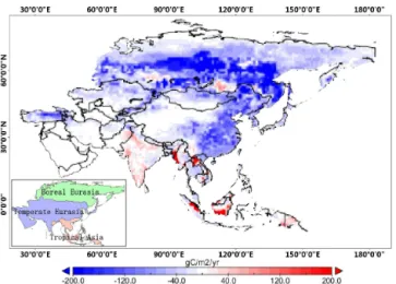
Figure 3. Mean terrestrial biosphere carbon flux estimated from our system over Asia during the period from 2006–2010 at a 1×1 grid resolution. Blue colors (negative) denote net carbon uptake while red colors (positive) denote carbon release to the atmosphere. Note that the estimated flux map includes net terrestrial fluxes and biomass-burning sources but excludes fossil fuel emissions.
3.2 Inverted Asian terrestrial CO2flux
3.2.1 Five-year mean
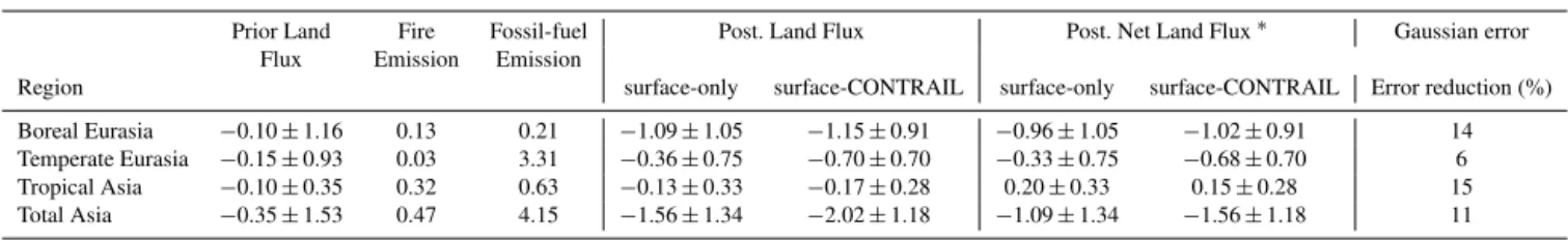
During the period from 2006–2010, we found a mean net terrestrial land carbon uptake (a posteriori) in Asia of −1.56 Pg C yr−1, consisting of −2.02 Pg C yr−1 uptake
by the terrestrial biosphere and+0.47 Pg C yr−1release by
biomass-burning (fire) emissions (Table 6). This terrestrial uptake compensates 38 % of the estimated+4.15 Pg C yr−1
CO2 emissions from fossil fuel burning and cement
man-ufacturing in Asia. An uncertainty analysis for the Asian terrestrial CO2 uptake derived from a set of sensitivity
ex-periments has been conducted and put the estimated sink in a range from−1.07 to−1.80 Pg C yr−1 (Table 3), while
the 1-sigma of the formal Gaussian uncertainty estimate is
±1.18 Pg C yr−1 (Table 6). The estimated Asian net
terres-trial CO2 sink is further partitioned into a−1.02 Pg C yr−1
carbon sink in boreal Eurasia and a −0.68 Pg C yr−1
car-bon sink in temperate Eurasia, with a+0.15 Pg C yr−1CO2
source in tropical Asia.
The annual mean spatial distribution of net terrestrial car-bon uptake over Asia is shown in Fig. 3. Note that the es-timated fluxes include terrestrial fluxes and biomass-burning sources but exclude fossil fuel emissions. Most Asian regions were natural carbon sinks over the studied period, with the strongest carbon uptake in the middle and high latitudes of the Northern Hemispheric part of Asia, while the low-latitude region releases CO2to the atmosphere. This flux distribution
pattern is quite consistent with previous findings that north-ern temperate and high latitude ecosystems were large sinks
−0.6 −0.5 −0.4 −0.3 −0.2 −0.1 0 0.1
CO2 fluxes (Pg C/yr)
Conifer ForestBroadleaf ForestMixed ForestGrass/ShrubTropical ForestSemitundraFields/Woods/SavannNorthern TaigaForest/FieldWetlandCrops Water
Case 1 (surface−CONTRAIL) Case 2 (surface−only)
Figure 4.Fluxes per ecoregion in Asia averaged over the period 2006–2010 in Cases 1 and 2 (in Pg C yr−1).
(Hayes et al., 2011) and tropical land regions were carbon sources (Gurney et al., 2003).
The aggregated terrestrial CO2fluxes 19 different
ecosys-tems (Fig. 1a) averaged over the period 2006–2010 are shown in Tables 4 and 5 and Fig. 4 (see Case 1). The ma-jority of the carbon sink was found in the regions domi-nated by forests, crops and grass/shrubs. The largest uptake is by the forests with a mean sink of−0.77 Pg C yr−1, 83 %
of which (−0.64 Pg C yr−1)was taken up by conifer forests
and 18 % of which (−0.14 Pg C yr−1) by mixed forest,
whereas the tropical forests released CO2(+0.08 Pg C yr−1).
The estimated flux by CTDAS in Asian cropland ecosys-tems was −0.20 Pg C yr−1, with the largest crop carbon
sink located in temperate Eurasia (−0.17 Pg C yr−1). The grass/shrub lands in Asia absorbed −0.44 Pg C yr−1, with
most of these grass/shrub sinks located in temperate Eura-sia (−0.36 Pg C yr−1). Other land-cover types (e.g., wetland, semi tundra and so on) sequestered about−0.15 Pg C yr−1
(10 % of total) over Asian regions. This suggests that accord-ing to our model, many ecosystems contributed to Asian CO2
sinks, highlighting the complexity of the total northern hemi-spheric sinks.
Also, we note that the detailed CO2flux partitioning in our
assimilation system highly relies on the prior model descrip-tion of the ecosystem-by-ecosystem flux patterns. To evalu-ate the Gaussian errors of the CO2flux estimate for a related
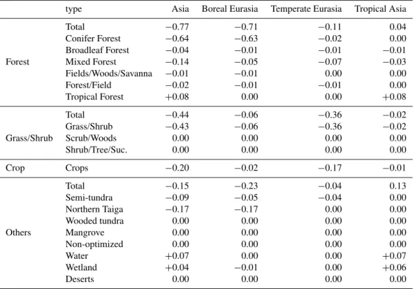
ecosystem types are to some extent constrained by the as-similation system. However, a large uncertainty still exists in the posterior carbon sink for most ecosystem types.We can make the assumption that the correlation between two inverted ecosystem-related fluxes indicates how well the ecosystem-related estimation of carbon fluxes is being strained by the observations (lower correlation, stronger con-strained; while higher correlation, weaker constrained), to further explore the optimized carbon fluxes during the period 2006–2010 (data shown in Table 4). As shown in Fig. 5, the absolute values of posterior correlation coefficients are less than 0.5 (most in the range of−0.3 to 0.5), while they started
uncorrelated (0.0). This confirms that ecoregion fluxes have not been fully independently retrieved.
3.2.2 Seasonal variability
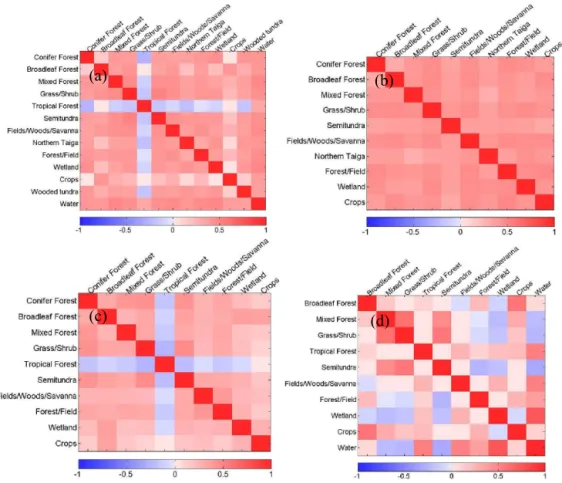
Figure 6 shows the prior and posterior seasonal cycles of CO2 fluxes for the Asia region and its three sub-regions as
well as their Gaussian uncertainties. The seasonal amplitude in boreal Eurasia as shown in Fig. 6b proves to be the ma-jor contributor to the seasonal signal in Asia (Fig. 6a). The large uptake of boreal Eurasia occurs in summer and the large differences between the prior and the posterior fluxes are also found in the summer growing season, indicating the surface observation network and CONTRAIL data largely affect the estimated fluxes. Our monthly variability is very close to changes in boreal Eurasia presented by Gurney et al. (2004). In Fig. 6c, the seasonal pattern for the temperate Eurasia region shows a comparable pattern to boreal Eurasia but with a smaller seasonal magnitude. And the adjustments of the prior flux in spring and summer are also smaller. The largest CO2uptake in temperate Eurasia subregion, however,
is shifted from July to August compared to boreal Eurasia, suggesting that a phase shift in the growing season occurred here with the highest CO2 sink occurring later in the year.
This seasonal cycle is slightly different from that reported by Gurney et al. (2004), but shows a nice agreement with the seasonal dynamics of Niwa et al. (2012) in the Southern tem-perate Asia region, and of Patra et al. (2011) in the Northwest Asia region. In tropical Asia (Fig. 6d), the seasonal variation is very different from other Asian subregions characterized by a weak CO2 uptake peak in August–October and much
smaller carbon release in May–July. Overall, the posterior uncertainty reduction for the period 2006–2010 was about 25 % in Asia, with the largest uncertainty remaining in the summer, suggesting that our model may not fully capture the biosphere sink signal in the growing season.
3.2.3 Interannual variability (IAV)
Figure 7 shows the estimated annual cumulative net ecosys-tem exchange in Asia during the period from 2006–2010 as well as its anomaly with weekly intervals. Here, the biomass-burning and fossil fuel emissions are excluded, and only the
sum of fluxes from respiration and photosynthesis are shown, because biomass-burning emissions have large interannual variability, especially for tropical Asia.
The coefficient of IAV (IAV=standard deviation/mean) in Asian land carbon flux is 0.12, with a peak-to-peak amplitude of 0.57 Pg C yr−1(amplitude=smallest – largest CO2sink),
ranging from the smallest carbon uptake of−1.71 Pg C yr−1
in 2010 and the largest CO2sink of−2.28 Pg C yr−1in 2009.
As has been noted in many other studies (Gurney et al., 2004, 2008; Mohammat et al., 2012; Patra et al., 2011; Peters et al., 2007, 2010; Yu et al., 2013), the IAV of the carbon flux strongly correlates with climate factors, such as air tempera-ture, precipitation and moisture.
The year 2010 stands out as a particularly low up-take year in Asia, with a reduction of terrestrial upup-take of 0.31 Pg C yr−1 compared to the five-year mean. This
re-duction mainly appeared in temperate Eurasia and ropical Asia, leading to+0.25 Pg C yr−1(35 % sink reduction) and +0.04 Pg C yr−1 flux anomalies (24 % sink reduction) in their corresponding regions. In 2010, Asia experienced a set of anomalous climate events. For example, temperate Eura-sia experienced a severe spring/autumn drought, and a heavy summer flood and a heat wave occurred in 2010 (National Climate Center, 2011). From Fig. 7b, we can see that 2010 did not show large anomalies until after the spring growing season. As anomalous climate appeared, the summer flood and autumn drought were identified as dominant climatic factors controlling vegetation growth and exhibiting a sig-nificant correlation with the land carbon sink, particularly in the croplands, grasslands and forests of temperate Eurasia. In the end, 2010 only showed−1.71 Pg C yr−1biospheric CO
2
uptakes (excluding fires) by the end of the year.
In contrast to 2010, the year 2009 had the strongest carbon sink for the study period, with much stronger uptake in tem-perate Eurasia (−0.20 Pg C yr−1 anomaly, 28 % increase in
CO2 uptake) as well as in boreal Eurasia (−0.05 Pg C yr−1
anomaly, 4 % uptake increase compared to the five-year mean). It can be seen that 2009 started with a lower-than-average release of carbon in the first 4 months (17 weeks) of the year amounting to+0.28 Pg C yr−1 compared to the
five-year average of+0.45 Pg C yr−1. This variation of the
Asian terrestrial carbon sink in the spring vegetation grow-ing season may partly relate to a higher sprgrow-ing temperature in 2009 which induced an earlier onset of the growing sea-son and led to a high vegetation productivity by extending the growing season (Mohammat et al., 2012; Richardson et al., 2009; Walther et al., 2002; Wang et al., 2011; Yu et al., 2013). From Fig. 7b, 2009 shows a very high carbon uptake in the summer growing season (June–August, weeks 22 to 32) concurrent with favorable temperature and abundant pre-cipitation conditions. After this summer, the vegetation pro-ductivity returned back to normal and the total cumulative carbon sink added up to−2.28 Pg C yr−1at the end of the
year with−0.26 Pg C yr−1extra uptake compared to the
5816 H. F. Zhang et al.: Estimating Asian terrestrial carbon fluxes
Table 4.The ecosystem-type associated posterior terrestrial biosphere fluxes for 2006–2010 (units of Pg C yr−1).
type Asia Boreal Eurasia Temperate Eurasia Tropical Asia
Total −0.77 −0.71 −0.11 0.04
Conifer Forest −0.64 −0.63 −0.02 0.00 Broadleaf Forest −0.04 −0.01 −0.01 −0.01 Forest Mixed Forest −0.14 −0.05 −0.07 −0.03 Fields/Woods/Savanna −0.01 −0.01 0.00 0.00 Forest/Field −0.02 −0.01 −0.01 0.00 Tropical Forest +0.08 0.00 0.00 +0.08
Total −0.44 −0.06 −0.36 −0.02 Grass/Shrub −0.43 −0.06 −0.36 −0.02 Grass/Shrub Scrub/Woods 0.00 0.00 0.00 0.00 Shrub/Tree/Suc. 0.00 0.00 0.00 0.00
Crop Crops −0.20 −0.02 −0.17 −0.01
Total −0.15 −0.23 −0.04 0.13
Semi-tundra −0.09 −0.05 −0.04 0.00 Northern Taiga −0.17 −0.17 0.00 0.00 Wooded tundra 0.00 0.00 0.00 0.00
Others Mangrove 0.00 0.00 0.00 0.00
Non-optimized 0.00 0.00 0.00 0.00
Water +0.07 0.00 0.00 +0.07
Wetland +0.04 −0.01 0.00 +0.06
Deserts 0.00 0.00 0.00 0.00
Table 5.The posterior/prior Gaussian errors (1-sigma) as well as the error reduction rate for the ecosystem types for 2006–2010.
type Posterior(Prior) Gaussian errors (Pg C yr−1) Gaussian error reduction rate (%)∗ Asia Boreal Temperate Tropical Asia Boreal Temperate Tropical
Eurasia Eurasia Asia Eurasia Eurasia Asia Total 0.81(1.07) 0.74(0.98) 0.22(0.28) 0.26(0.31) 24.30 % 24.49 % 21.43 % 16.13 % Conifer Forest 0.71(0.94) 0.71(0.94) 0.05(0.06) 0(0) 25.43 % 25.53 % 16.33 % – Broadleaf Forest 0.12(0.14) 0.05(0.06) 0.1(0.12) 0.04(0.04) 14.29 % 16.67 % 16.67 % 0.00 % Forest Mixed Forest 0.27(0.33) 0.21(0.25) 0.16(0.2) 0.04(0.05) 18.18 % 16.00 % 20.00 % 20.00 % Fields/Woods/Savanna 0.11(0.14) 0.05(0.06) 0.10(0.13) 0.01(0.02) 12.43 % 11.67 % 12.08 % 11.00 % Forest/Field 0.10(0.12) 0.08(0.09) 0.04(0.06) 0.05(0.06) 16.67 % 11.11 % 33.33 % 16.67 % Tropical Forest 0.25(0.30) 0(0) 0.05(0.06) 0.25(0.3) 16.67 % – 16.67 % 16.67 % Total 0.48(0.63) 0.17(0.2) 0.45(0.59) 0.05(0.06) 23.81 % 21.85 % 14.73 % 22.67 % Grass/Shrub 0.48(0.63) 0.17(0.2) 0.45(0.59) 0.05(0.06) 23.81 % 21.85 % 14.73 % 22.67 % Grass/Shrub Scrub/Woods 0(0) 0(0) 0(0) 0(0) – – – – Shrub/Tree/Suc. 0(0) 0(0) 0(0) 0(0) – – – – crop Crops 0.48(0.63) 0.09(0.11) 0.46(0.61) 0.1(0.12) 23.81 % 18.18 % 24.59 % 16.67 % Total 0.52(0.64) 0.48(0.6) 0.19(0.23) 0.02(0.02) 18.75 % 20.00 % 17.39 % 0.00 % Semi-tundra 0.35(0.43) 0.3(0.36) 0.19(0.23) 0(0) 18.60 % 16.67 % 17.39 % – Northern Taiga 0.36(0.45) 0.36(0.45) 0(0) 0(0) 20.00 % 20.00 % – – Wooded tundra 0(0) 0(0) 0(0) 0(0) – – – – Others Mangrove 0(0) 0(0) 0(0) 0(0) – – – – Non-optimized 0(0) 0(0) 0(0) 0(0) – – – – Water 0.00(0.00) 0(0) 0(0) 0.00(0.00) 8.70 % – – 8.70 % Wetland 0.1(0.12) 0.10(0.12) 0.0(0.0) 0.02(0.02) 16.67 % 11.67 % 11.40 % 18.00 % Deserts 0(0) 0(0) 0(0) 0(0) – – – –
∗Gaussian error reduction rate is calculated as follows:(σ
(a) (b)
(c) (d)
Figure 5.The matrixes of the ecosystem-by-ecosystem paired correlations for the optimized carbon fluxes during the period 2006–2010 are (a)Asia;(b)boreal Eurasia;(c)temperate Eurasia;(d)tropical Asia.
3.2.4 Uncertainty estimation
Table 3 presents the estimated annual mean NEE across the alternative sensitivity experiments. The time spans are dif-ferent among six tests. Case 1 (surface-CONTRAIL) and Case 2 (surface-only) run for the period 2006–2010 (the pe-riod 2004–2005 servers as a spin-up pepe-riod), while Cases 3 to 6 run for the period 2008–2010. To compare other alter-native sensitivity estimates for the same period from 2008– 2010, we calculated this three-year average of annual Asia CO2fluxes (the period 2008–2010) from all the six tests to
be−1.61,−1.15,−1.69,−1.80,−1.23 and−1.07 PgC yr−1,
respectively. The Asian CO2uptake thus ranges from−1.07
to−1.80 Pg C yr−1across our sensitivity experiments, which
complements the Gaussian error. Despite the small num-bers of years included, this range suggests that the Asian terrestrial was a sizable sink, while a carbon source im-plied in previous studies by the 1-sigma Gaussian error of
±1.18 Pg C yr−1 on the estimated mean, is very unlikely.
The largest sensitivity in inferred flux is to the change of prior terrestrial biosphere fluxes (Case 4, difference=Case 4
– Case 1). The inversions with different model resolutions (Case 5, difference =Case 5 – Case 2) and with different
Chinese fossil fuel emissions (Case 3, difference =Case 4
– Case 1) also show large variations in the inverted CO2
fluxes, while the sensitivity to the change of land cover types (Case 6, difference=Case 6 – Case 2) is generally modest. This highlights the current uncertainties in the Asian sink and the best method to estimate it from inverse modeling.
3.2.5 Impacts of the CONTRAIL data on inverted Asian CO2flux
We examined the impacts of the CONTRAIL data on Asian flux estimation by comparing results from Case 1 (surface-CONTRAIL) and Case 2 (surface-only) (Table 6 and Fig. 8a). Note that the uncertainties shown in the Table 6 and Fig. 8b are now the Gaussian uncertainties as we did not repeat all sensitivity experiments. As shown in Table 6, inclu-sion of the CONTRAIL data induces an averaged extra CO2
sink of about−0.47 Pg C yr−1to Case 1 (0.47=1.56–1.09),
with most addition to the grass/shrub ecosystem (Fig. 4). The spatial pattern of Asian fluxes also changed considerably (see Fig. 8a). For instance, a decrease in CO2uptake was found
5818 H. F. Zhang et al.: Estimating Asian terrestrial carbon fluxes
2 4 6 8 10 12
−20 −15 −10 −5 0 5
CO2 fluxes (Pg c/yr)
Fluxes time series of Asia
Prior posterior
2 4 6 8 10 12
−15 −10 −5 0 5
Fluxes time series of Boreal Eurasia
2 4 6 8 10 12
−6 −4 −2 0 2
Fluxes time series of Temperate Eurasia
CO2 fluxes (Pg c/yr)
month
2 4 6 8 10 12
−1 −0.5 0 0.5
Fluxes time series of Tropical Asia
month
(d) (c)
(a) (b)
Figure 6.A priori and posteriori averaged fluxes (with uncertain-ties) over Asian regions during the period 2006–2010 are listed as follows: (a) Asia; (b) boreal Eurasia; (c) temperate Eurasia; (d)tropical Asia. This flux is biosphere carbon sink after removal of fossil and biomass-burning fluxes.
Jan−30 Mar−06 Apr−10 May−15 June−19 July−24 Aug−28 Oct−02 Nov−06 Dec−11 −3
−2.5 −2 −1.5 −1 −0.5 0 0.5
Aggregated flux(Pg C)
2006 (−1.84) 2007 (−2.21) 2008 (−2.06) 2009 (−2.28) 2010 (−1.71) mean (−2.02)
0 5 10 15 20 25 30 35 40 45 50 55
−0.5 −0.4 −0.3 −0.2 −0.1 0 0.1 0.2 0.3
week of year
Aggregated flux anomaly(Pg C)
2006 (0.18) 2007 (−0.19) 2008 (−0.04) 2009 (−0.26) 2010 (0.31)
(b) (a)
Figure 7. (a)Cumulative net Asian ecosystem exchange (NEE) vs. time estimated in our system for each of the individual years and for the 2006–2010 mean. This figure reveals the largest uptake in 2009 and the smallest uptake in 2010.(b)Cumulative anomaly of Asian CO2exchange through the years 2006 to 2010. The inferred Asian
carbon fluxes shown here include only respiration and photosyn-thesis, because the biomass-burning emissions have a large inter-annual variability.
Figure 8. (a)The inverted flux difference between surface CO2 observation data only surface (surface-only) and both the surface CO2observation data and CONTRAIL data (surface-CONTRAIL); and(b)the Gaussian error reduction rate between surface-only and surface-CONTRAIL during the period 2006–2010. The flux differ-ence is derived from (surface-CONTRAIL – surface-only), while the Gaussian error reduction rate is calculated as(σsurface−only− σsurface−CONTRAIL)/σsurface−only×100.
distribution in tropical Asia showed a small spatial change and a large increase in regional sink size with CONTRAIL observations included.
Table 6 and Fig. 8b shows the reduction of the Gaussian error between Case 1 and Case 2. The error reduction rate (ER) is calculated as the following percentage:
ER=(σsurface−only−σsurface−CONTRAIL) σsurface−only×100
, (2)
whereσsurface−onlyandσsurface−CONTRAILare Gaussian errors
Table 6.The prior/posterior land fluxes, biomass-burning (fire) emissions, fossil fuel emissions and net land flux as well as the Gaussian error/their error reduction rates in surface-only and surface-CONTRAIL inversion experiments during the period 2006–2010 (in Pg C yr−1).
Prior Land Fire Fossil-fuel Post. Land Flux Post. Net Land Flux∗ Gaussian error
Flux Emission Emission
Region surface-only surface-CONTRAIL surface-only surface-CONTRAIL Error reduction (%)
Boreal Eurasia −0.10±1.16 0.13 0.21 −1.09±1.05 −1.15±0.91 −0.96±1.05 −1.02±0.91 14
Temperate Eurasia −0.15±0.93 0.03 3.31 −0.36±0.75 −0.70±0.70 −0.33±0.75 −0.68±0.70 6
Tropical Asia −0.10±0.35 0.32 0.63 −0.13±0.33 −0.17±0.28 0.20±0.33 0.15±0.28 15
Total Asia −0.35±1.53 0.47 4.15 −1.56±1.34 −2.02±1.18 −1.09±1.34 −1.56±1.18 11
∗
Posterior Net Land Flux including posterior land flux and fire emissions, but excluding fossil emissions.
Asia (reducing by 14 % and 15 %, respectively). This sug-gests that current surface CO2observations data alone do not
sufficiently constrain these regional flux estimations (there are no observation sites in boreal Eurasia and only one in tropical Asia), and the additional CONTRAIL CO2
observa-tions impose an extra constraint that can help reduce uncer-tainty on inferred Asia CO2fluxes, especially for these two
surface observation sparse regions.
4 Discussions and conclusions
4.1 Impact of CONTRAIL
Our modeling experiments reveal that the extra aircraft ob-servations shift the inverted CO2 flux estimates by
impos-ing further constraints. This confirms the earlier findimpos-ings by Saeki et al. (2003) and Maksyutov et al. (2013) that the in-verted fluxes were sensitive to observation data used. For tropical Asia, inclusion of the CONTRAIL data notably re-duced the uncertainties (about 15 % reduction). Compared with an inversion study with the CONTRAIL data for the tropical Asia region (Niwa et al., 2012) , the error reduction rate in land flux estimation in this study for the same region is smaller than that of Niwa et al. (34 %). This difference in uncertainty reduction likely results from the differences in inversion system design between these two studies, of which vertical mixing represented in transport model, and covari-ance assigned to prior fluxes are typically most important. We furthermore note that the set of observations used in these studies was not identical, we for instance included one trop-ical surface site (BKT, see Table 1 and Fig. 1a) to constrain the inferred flux estimation but Niwa, et al. (2012) did not.
Our results share other features with the Niwa et al. (2012) study, for instance the largest impact on the least data con-strained regions. As reported by Niwa et al. (2012), the in-clusion of CONTRAIL measurements not only constrains the nearby fluxes, but also reduces inferred flux errors in the re-gions far from the CONTRAIL measurement locations. For instance, in boreal Eurasia, where no surface site exists and which is far from the CONTRAIL data locations (after pre-processing of horizontal/vertical bins and filter operation of stratospheric, there is no CONTRAIL observation available over this region), uncertainty reductions are large (14 %
re-duction in uncertainty). Similar results were also presented by Niwa et al. (2012), with an 18 % error reduction in bo-real Eurasia. These two studies consistently suggest that in-cluding the CONTRAIL measurements in inversion model-ing systems will help to increase the NEE estimation accu-racy over boreal Eurasia.
The CONTRAIL constraint on temperate Eurasia is gen-erally modest, only having a 6 % error reduction. This may because temperate Eurasia has more surface observation sites than other regions in Asia. However, it is interesting that the difference in inverted NEE in this region between surface-only and surface-CONTRAIL is large (−0.35 Pg C yr−1), but inconsistent with Niwa et al. (2012). One cause of this is likely the sensitivity of these inverse systems to vertical transport (Stephens et al., 2007), as also suggested by Niwa et al. (2012). The uneven distribution of observations at the surface and free troposphere may also aggravate this discrep-ancy.
4.2 Comparison of the estimated Asian CO2flux with other studies
Our estimated Asian terrestrial carbon sink is about
−1.56 Pg C yr−1 for the period 2006–2010. Most parts of
Asian were estimated to be CO2sinks, with the largest
car-bon sink (−1.02 Pg C yr−1) in boreal Eurasia, a second large
CO2 sink (−0.68 Pg C yr−1) in temperate Eurasia, and a
small source (+0.15 Pg C yr−1) in tropical Asia. This spa-tial distribution of estimated terrestrial CO2 fluxes is
over-all comparable to the results for the period of 2000–2009 by Saeki et al. (2013), derived from an inversion approach fo-cusing on Siberia with additional Siberian aircraft and tower CO2measurements, especially in the high latitude areas.
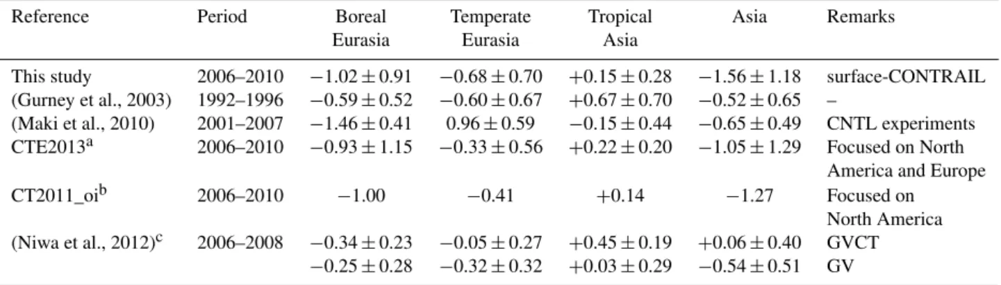
Comparisons of our inverted CO2flux with previous
stud-ies are summarized in Table 7. In boreal Eurasia, our in-ferred land flux (−1.02 Pg C yr−1) is higher than Gurney
et al. (2003) (−0.59 Pg C yr−1 during the period 1992–
1996), but close to Maki et al. (2010) (−1.46 Pg C yr−1
during the period 2001–2007), CTE2013 (−0.93 Pg C yr−1)
and CT2011_oi (−1.00 Pg C yr−1, downloaded from http:
//carbontracker.noaa.gov). In Temperate Eurasia, our in-verted flux is −0.68 Pg C yr−1, which is well
5820 H. F. Zhang et al.: Estimating Asian terrestrial carbon fluxes
Table 7.Comparison of the inverted Asia terrestrial ecosystem carbon fluxes (in Pg C yr−1)from this study with previous studies.
Reference Period Boreal Temperate Tropical Asia Remarks Eurasia Eurasia Asia
This study 2006–2010 −1.02±0.91 −0.68±0.70 +0.15±0.28 −1.56±1.18 surface-CONTRAIL (Gurney et al., 2003) 1992–1996 −0.59±0.52 −0.60±0.67 +0.67±0.70 −0.52±0.65 –
(Maki et al., 2010) 2001–2007 −1.46±0.41 0.96±0.59 −0.15±0.44 −0.65±0.49 CNTL experiments CTE2013a 2006–2010 −0.93±1.15 −0.33±0.56 +0.22±0.20 −1.05±1.29 Focused on North
America and Europe CT2011_oib 2006–2010 −1.00 −0.41 +0.14 −1.27 Focused on
North America (Niwa et al., 2012)c 2006–2008 −0.34±0.23 −0.05±0.27 +0.45±0.19 +0.06±0.40 GVCT
−0.25±0.28 −0.32±0.32 +0.03±0.29 −0.54±0.51 GV
aCTE2013: Carbon Tracker Europe in Peylin et al. (2013) for the period 2006–2010.bCT2011_oi: download from http://carbontracker.noaa.gov; without providing
uncertainties; Note that that the CTE2013 and CT2011_oi estimates are not independent, and share the TM5 transport model and ObsPack observations sets, but differences in zoomed transport, state vector configuration and prior biosphere models used.cGVCT: jointly using GLOBALVIEW and CONTRAIL CO2observation
data to perform inversion; GV: only GLOBALVIEW data used to conduct inversion; Note that the numbers of boreal Eurasia and temperate Eurasia and were obtained by personal communication.
Table 8.Comparison of IAVs of the terrestrial ecosystem carbon fluxes in Asia during the period 2006–2010 from this study with previous studies. Fluxes (in Pg C yr−1)include biomass-burning emissions but exclude fossil fuel emissions.
year Boreal Eurasia Temperate Eurasia Tropical Asia This study CTE2013 This study CTE2013 This study CTE2013
2006 −0.93 −0.93 −0.6 −0.4 0.37 0.41 2007 −1.17 −0.88 −0.8 −0.44 0.14 0.18 2008 −0.96 −1.07 −0.66 −0.33 −0.09 0.00 2009 −1.04 −0.78 −0.88 −0.34 0.12 0.25 2010 −1.01 −1.02 −0.49 −0.12 0.19 0.27
(−0.41 Pg C yr−1)even though we used a similar inversion framework. One reason of this discrepancy is likely that dif-ferent zoomed regions were configured in the inversion sys-tem. Another main factor is likely the inclusion of CON-TRAIL largely impacts on our Temperate Eurasia’s carbon estimates. In tropical Asia, our estimate is+0.15 Pg C yr−1,
which is in the range of Niwa et al. (2012) (+0.45 Pg C yr−1,
GVCT) and Patra et al. (2013) (−0.104 Pg C yr−1), both in-cluding aircraft CO2 measurements in their inversion
mod-eling, and very close to the CTE2013 (+0.22 Pg C yr−1)
and CT2011_oi (+0.14 Pg C yr−1). The estimated total Asian terrestrial carbon sink is −1.56 Pg C yr−1, which is
close to the CTE2013 (−1.05 Pg C yr−1) and CT2011_oi
(−1.27 Pg C yr−1). The IAVs comparison between the results
from this study and from CTE2013 is also presented in Ta-ble 8 (different from IAV in Sect. 3.2.2, these results include biomass-burning emissions). The IAVs are different between inferred terrestrial CO2flux of this study and CTE2013. In
boreal Eurasia, there was a moderate Asian CO2 sink in
2007 for CTE2013, while the results from this study show the highest carbon uptake for this year; in CTE2013, the strongest terrestrial CO2sink occurs in 2008, while from our
estimates the sink in 2008 was weaker than that in 2007. For temperate Eurasia, the highest land sink occurs in 2007 for
CTE2013, while in this study, the highest occurs in 2009. In tropical Asia, there is very similar IAVs between CTE2013 and this study, but the size of the carbon sink is inconsis-tent. Differences likely stems from the additions of Asian sites and CONTRAIL data in this study. Compared to pre-vious findings, our updated estimation with these additional data seems to support a larger Asian carbon sink over the past decade.
The spatial patterns of NEE in Asia are complex because of large land surface heterogeneity, such as land cover, veg-etation growth rates, soil types, and varying responses to cli-mate variations. This makes accurately estimating NEE over Asia challenging. We believe this study is therefore useful to improve our understanding of the Asia regional terrestrial carbon cycle even though our estimation still has remaining uncertainties and biases in the inverted fluxes. By these com-parisons, we can also conclude that our inferred Asia land surface CO2fluxes support a view that both large boreal and
mid-latitude carbon sinks in Asia are balanced partly by a small tropical source. This would support the earlier sugges-tion that Asia is of key interest to better understand the global terrestrial carbon budget in the context of climate change.
The majority of the CO2sink was found in the areas
not all individually constrained by the observations. Asian forests were estimated to be a large sink (−0.77 Pg C yr−1)
during the period 2006–2010, the sink size is slightly larger than the bottom-up derived results of Pan et al. (2011) (−0.62 Pg C yr−1)for the period 1990–2007. One cause of this discrepancy is likely due to that our estimate is pre-sented at a coarse resolution (a 1◦×1◦ grid may contain
other biomes with lower carbon uptake than forests). Another reason may be that about half of Temperate Eurasia was not included in the statistical analysis by Pan et al. (2011). Note that the carbon accumulation in wood products is not con-sidered in our estimates and needs further analysis in future studies.
The croplands in Asia were identified to be an average sink of−0.20 Pg C yr−1during the period 2006–2010. The uptake
in croplands is likely associated with agricultural technique and crop management. Different from other natural ecosys-tems, crop ecosystems are usually under intensive farming cultivation, with regular fertilizing and irrigation of the crops. This increases crop production, and in return leads to high residues and root to the soil, which increases the carbon sink in cropland (Chen et al., 2013). However, the accumulation of crop carbon in most crop ecosystems is relatively low, and agricultural areas are even considered not to contribute to a long-term net sink (Fang et al., 2007; Piao et al., 2009; Tian et al., 2011). This is because the carbon accumulation in the crop biomass is harvested at least once per year and released back as CO2to the atmosphere after consumption. We should
note that our estimate in the crop sink is different from the re-sults of “crop no contribution ” (Piao et al., 2009). Our atmo-spheric inversion system can well capture the crop’s strong CO2uptake during the growing season, but the atmosphere
locally does not reflect the emission of the harvested crops, which normally have been transported laterally and is con-sumed elsewhere. This harvested product is likely released from a region with high population density and hard to de-tect against high fossil fuel emissions, whereas the estimated crop flux remains a large net CO2 uptake over the period
considered even though the crop flux into the soil is rela-tively small. Thus the croplands’ sink in this study might be overestimated due to the absence of harvesting in our model-ing system. This issue was also raised by Peters et al. (2007, 2010).
Grassland/Shrub ecosystems also play an important role in the global carbon cycle, accounting for about 20 % of to-tal terrestrial production and could be a potential carbon sink in future (Scurlock and Hall, 1998). The grass/shrub lands in Asia absorbed a total of−0.44 Pg C yr−1, accounting for
about 25 % of the total Asian terrestrial CO2 sink, which
is close to the averaged global grassland sink percentage of 20 %. Compared to the bottom-up results that net ecosystem productivity was 10.18 g C m−2yr−1by Yu et al. (2013), our estimate of 34.32 g C m−2yr−1 is much higher. This might be due to the fact that the areas in this study include shrubs, whereas other studies only consider grasslands.
The Supplement related to this article is available online at doi:10.5194/acp-14-5807-2014-supplement.
Acknowledgements. We wish to thank the Y. Niwa of
Geochem-ical Research Department, MeteorologGeochem-ical Research Institute, Tsukuba, Japan for providing many important comparable results and useful comments on this study. We kindly acknowledge all atmospheric data providers to the ObsPack version 1.0.2, and those that contribute their data to WDCGG. We are grateful to M. Ramonet of French RAMCES (Réseau Atmosphérique de Mesure des Composés à Effet de Serre), A. J. Gomez-Pelaez of Izaña Atmospheric Research Center (IARC), Meteorological State Agency of Spain (AEMET), Spain, B. Stephens of NCAR, L. Haszpra of Hungarian Meteorological Service and S. Hammer of University of Heidelberg, Institut fuer Umweltphysik for CO2time series used in this assimilation system. This research is supported by a research grant (2010CB950704) under the Global Change Program of the Chinese Ministry of Science and Technology, the Strategic Priority Research Program “Climate Change: Carbon Budget and Related Issues” of the Chinese Academy of Sciences (XDA05040403), the National High Technology Research and Development Program of China (Grant no. 2013AA122002),the research grant (41271116) funded by the National Science Founda-tion of China, a Research Plan of LREIS (O88RA900KA), CAS, a research grant (2012ZD010) of Key Project for the Strategic Science Plan in IGSNRR, CAS, and “One Hundred Talents” program funded by the Chinese Academy of Sciences. Wouter Peters was supported by an NWO VIDI Grant (864.08.012) and the Chinese-Dutch collaboration was funded by the China Exchange Program project (12CDP006). I. van der Laan-Luijkx has received funding from the European Union’s Seventh Framework Programme (FP7/2007–2013) under grant agreement no. 283080, project GEOCARBON.
Edited by: R. Keeling
References
Baker, D., Law, R., Gurney, K., Rayner, P., Peylin, P., Den-ning, A., Bousquet, P., Bruhwiler, L., Chen, Y. H., and Ciais, P.: TransCom 3 inversion intercomparison: Impact of trans-port model errors on the interannual variability of regional CO2fluxes, 1988–2003, Global Biogeochem. Cy., 20, GB1002,
doi:10.1029/2004GB002439, 2006.
Boden, T., Marland, G., and Andres, R.: Global, regional, and national fossil-fuel CO2 emissions, Carbon Dioxide In-formation Analysis Center, Oak Ridge National Labora-tory, US Department of Energy, Oak Ridge, Tenn., USA doi:10.3334/CDIAC/00001_V2011, 10, 2011.
Broquet, G., Chevallier, F., Bréon, F.-M., Kadygrov, N., Alemanno, M., Apadula, F., Hammer, S., Haszpra, L., Meinhardt, F., Morguí, J. A., Necki, J., Piacentino, S., Ramonet, M., Schmidt, M., Thompson, R. L., Vermeulen, A. T., Yver, C., and Ciais, P.: Re-gional inversion of CO2ecosystem fluxes from atmospheric