Abstract— This paper describes a model for the analysis of multilay-ered chiral structures containing planar electric and magnetic scattering elements of arbitrary shape, illuminated by an elliptically polarized plane wave. The particular case of a single chiral layer is analyzed and the scattering matrices for single and dual electric and/or magnetic dipole distributions are derived in an original way. As an application, the polarimetric response of a short electric or magnetic dipole is directly obtained from their scattering matrix.
Index Terms— Chiral medium, electromagnetic scattering, Green’s functions, layered media, radar remote sensing, spectral fields.
I. INTRODUCTION
The development of polarimetric synthetic aperture radars (PolSAR) introduced new possibilities of
active microwave remote sensing of the Earth [1], [2]. By containing full amplitude and phase
information from each SAR image resolution cell, PolSAR signatures permit better target
discrimination and classification when compared to single-polarization SAR data, having thus been
successfully used for classification of a wide range of land cover [3], [4]. More recently, PolSAR
imaging techniques have also been applied to the analysis of man-made structures and urban areas,
despite the complexity added in these cases by the number and variety of elements involved in the
electromagnetic scattering [5], [6].
The problem of electromagnetic scattering and propagation in structures composed of multiple
layers of complex media appears often not only in microwave SAR remote sensing (e.g., stratified
soil, crop and forest vegetation, snow and ice covers), but also in other diverse applications, such as:
microstrip antennas, microwave monolithic integrated circuits (MMIC), printed circuit technology,
mobile and wireless communications, medical imaging and diagnosing, geophysical mapping and
planetary exploration. The efficient computational analysis of each of these cases requires accurate
models that account for the geometric and electromagnetic characteristics of the particular structure
under study, as well as for the specific electromagnetic excitation mechanism.
For practical PolSAR remote sensing applications, such as image classification and sensor
calibration, several models have been developed to properly characterize the electromagnetic
scattering of diverse targets [7]. For example, forest canopy models based on the Radiative Transfer
Scattering Analysis of Planar Electric and
Magnetic Dipoles in Multilayered Chiral
Structures
N. R. Rabelo, J. C. da S. Lacava, D. Fernandes
Laboratório de Antenas e Propagação, Instituto Tecnológico de Aeronáutica, Pr. Mal. Eduardo Gomes, 50 12228-900 São José dos Campos - SP, Brazil, {nrrabelo, lacava, david}@ita.br
S. J. S. Sant’Anna
(RT) theory have been largely utilized [8], providing good results when the medium consists of
sparsely distributed scatterers that are small compared to the wavelength of the incident radiation. In
this case, each scatterer needs to be carefully represented; a tree, for example, may be treated as a
cluster of elementary scattering elements: dielectric cylinders (representing its trunk and branches)
and smaller disks (for its leaves). On the other hand, taking into account the effect of multiple
scattering from rough surfaces or volumetric interactions is not a simple task. Therefore, for an
electrically dense medium, where scatterers are compactly distributed or the radiation frequency is
such that the spacing between them is comparable to the wavelength, the fundamental RT assumption
of independent scattering from the elements is no longer valid, thus requiring either complex model
adjustments or a different model altogether [9].
Another important consideration for the accuracy of a PolSAR remote sensing model is the
dielectric properties of the media that constitute each layer. Specialized literature reveals a variety of
such properties, for instance: natural media such as rocks, snow, and certain types of soil can not
usually be considered homogeneous [10]. Also, scattering from natural terrain cover can be strongly
anisotropic [11], as confirmed by measurements taken along different directions of the trunk, branches
and needles of certain conifers [12]. Still another example, chirality effects [13] have been observed in
radar remote sensing of certain types of vegetation [14].
Among the several different parameters used in the literature for polarimetric target
characterization, the scattering matrix, which combines both polarimetric and electromagnetic
properties of a given target, plays an important role. Once the scattering matrix for a given target is
accurately determined, other polarimetric target descriptors (e.g., its polarimetric response, radar cross
section, entropy, anisotropy, or terrain azimuth slope) can be derived as by-products of the scattering
matrix [1], [4].
In this context, the purpose of this article is twofold:
• To present a model for the analysis of scattering from planar electric and magnetic elements of
arbitrary shape embedded in a structure made out of multiple planar layers of chiral media, and
illuminated by an elliptically polarized plane wave at oblique incidence. The devised method is
based on the formalism previously developed for the study of scattering from multiple isotropic
planar layers [15], [16], with proven results in microstrip antenna and remote sensing
applications. The model for the isotropic structure has been extended to chiral media in a
formal and methodical way [17], though at the cost of added complexity, and allows for planar
electric and magnetic scattering elements of arbitrary shape.
• To derive from such model the scattering matrices associated with planar electric and magnetic
dipoles located at either one or both interfaces of a single chiral layer structure, resulting in
For achieving these purposes the paper is organized as follows. The theory behind the computation
of the electromagnetic fields present in the multilayered chiral structure is described in Section II. In
Section III the general chiral model is particularized for simple scattering elements (planar thin elec-
tric and magnetic dipoles) embedded in a three-layer planar structure consisting of a chiral layer
between free space and an isotropic ground. The scattering matrices for several configurations of
single and dual electric and/or magnetic dipoles are presented in Section IV. As applications of these
analytical results, the polarimetric response of electric and magnetic dipoles is discussed in Section V.
II. MULTILAYERED CHIRAL STRUCTURE MODEL
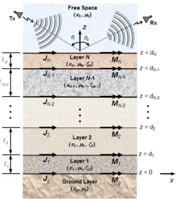
The general structure under investigation, as depicted in Fig. 1, consists of N chiral layers confined
in the z-direction between free space (the upper layer) and ground (the lower layer). The analytical
development is based on a global rectangular coordinate system located atop the ground layer (z=0).
All layers are assumed to be linear, homogeneous, planar and unbounded along the transversal x and y
directions. The isotropic ground layer, occupying the negative-z region, has complex permittivity εg and complex permeability μg, while free space, extending beyond z=dN, also isotropic, has permittivity ε0 and permeability μ0.
Fig. 1. Geometry of multilayered chiral structure (cut at plane y = 0).
A chiral medium corresponds [18] to a reciprocal bi-isotropic medium that is capable of supporting
two superimposed circularly-polarized waves, one to the left and the other to the right. Their different
propagation speeds introduce a phase difference in the propagation of these two waves. Thus, if a
plane, uniform, linearly-polarized electromagnetic wave is incident on a chiral medium, the observed
The n-th (for n=1, 2, … , N) chiral layer in Fig. 1 is characterized by permittivity εn, permeability μn, chiral admittance ζn, and thickness ℓn. Electric and magnetic elements of infinitesimal thickness are supposed to exist on each layer interface, i.e., at z=0 and z=dn, of the multilayered chiral structure.
The excitation mechanism consists of an elliptically polarized plane wave illuminating at oblique
incidence the z=dN interface between the uppermost chiral layer and free space. Considering the multilayered structure is located in the far range of the transmitting and the receiving antennas illustrated in
Fig.1, then the transmitted wave incident upon the z=dN interface and the scattered wave that reaches the receiving antenna can both be assumed to be plane and uniform [19]. Also, the elliptically polarized
excitation wave is represented as the superposition of two linearly polarized waves, one parallel to the
incidence plane (vertical polarization) and the other perpendicular to it (horizontal polarization).
The excitation wave induces on the electric and magnetic scattering elements located at the layer
interfaces electric and magnetic surface current densities, respectively expressed as Jξ(x,y)=xJξx(x,y) +yJξy(x,y) and Mξ(x,y)=xMξx(x,y)+yMξy(x,y), where boldface letters represent vectors, ξ∈{x,y},
and x and y are the unit vectors along the x- and the y-direction. These current densities are considered
the virtual sources of the electromagnetic field within each layer, as well as of the scattered field in
free space.
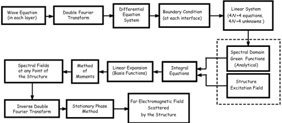
The electromagnetic field within any given layer is determined through the methodology described
in [17], whereby the structure is treated as a boundary value problem. The analysis is carried out in
the spectral domain using the full-wave technique, taking into account the surface electric and
magnetic current densities induced on the scattering elements. The solution for the electromagnetic
field in any of the N+2 layers, mathematically formulated in [17] and schematically depicted in the
block diagram on Fig. 2, can be summarized as follows:
• First, the wave equations for each of the N chiral layers, free space, and ground are solved in
the Fourier domain, resulting in a system of differential equations;
• Next, the application of the proper electromagnetic boundary conditions at each interface
yields a set of 4(N+1) equations in an equal numbers of unknowns, whose solution leads to
the spectral electric and magnetic Green's functions relating each of the N+2 layers;
• Then, the combination of the Green's functions and the spectral surface current densities
allows the determination of the spectral fields at any point of the multilayered structure;
• Finally, the electromagnetic fields in the spatial domain are obtained from the inverse double
Fourier transform.
For microwave remote sensing purposes, interest is in the analysis of the far electromagnetic field
scattered into free space by the multilayered structure. Since the scattered wave can be approximated
by a plane wave at the receiving antenna, considered sufficiently small, the stationary phase method [19] can
Fig. 2. Block diagram of the electromagnetic field computation method.
From these expressions and the knowledge of the current densities on the elements, the scattering matrix
is completely determined for any incidence and scattering direction. Using this method, the far scattered
electric field is expressed [19] in spherical coordinates by
}
{
( , ) ( , )cot 2
) , ,
( 0 0 0
0 0
0
φ θ z xe ye
ye xe z r
ik
k k k
k r
e ik
r θ η
π φ
θ ≅− − −
E (1)
where θ and φ are the unit vectors along the θ- and the φ-direction, η0 is the intrinsic impedance of free
space, k0 is the wavenumber in vacuum of the excitation wave, kxe=k0 sinθcosφ and kye=k0 sinθsinφ define the stationary phase point, r is the distance between the receiving antenna and the target, and 0z and
0z are the z-components of the spectral electromagnetic field in free space. As a remark, these components depend on the surface current densities induced on the elements, which can be determined by the method
of moments or other alternative techniques.
III. SCATTERING FROM A SINGLE CHIRAL LAYER STRUCTURE
In this section, the general case previously discussed is particularized for a single (i.e., N=1) chiral
layer with electric and magnetic currents on the interfaces z=0 and z=d (Fig. 3).
Fig. 3. Chiral layer between free space and ground.
Spectral Fields at any Point of the Structure
Differential Equation
System
Linear System (4N +4 equations,
4N +4 unknowns )
Far Electromagnetic Field Scattered by the Structure
Spectral Domain GreenFunctions
(Analytical) Method
of Moments
Inverse Double Fourier Transform
Stationary Phase Method Wave Equation
(in each layer)
Boundary Condition (at each interface) DoubleFourier
Transform
Structure Excitation Field Integral
Equations Linear Expansion
This simpler configuration is then represented by the following system of eight equations for the eight
longitudinal components of the spectral electromagnetic field, reflecting the coupling between the electric
and magnetic fields
gy y gx x gz g z z z
z ik ik ik k k
k
i + − + + =− m − m
− 11 2 2 3 3 4 4 ωµ (2a)
gy x gx y gz g z z z
z + + + − =k m −k m
γ γ γ γ
γ1 1 2 2 3 3 4 4 (2b)
gy y gx x gz g z z z
z k k k k k
k
q
{
1 1+ 2 2 + 3 3+ 4 4}
/(ωµ)−ωε = j + j (2c)gy x gx y gz g z z z
z k k
q
i
{
γ1 1−γ2 2 +γ3 3−γ4 4}
/(ωµ)−γ =− j + j (2d){
i d i dd
i i k e k e
e z z
z 0 1 1 1 2 2 2
0 0
γ γ
γ
ωµ − + − + + +
}
x x y y zz e k e k k
k i d i d
m m +
= +
− + 3 + 4
4 4 3 3 γ γ (2e) d i d i d
i e e
e z z
z 0 1 1 1 2 2 2
0 0
γ γ
γ γ γ
γ − + + + +
z e i d z e i d ky x kx y
m m +
− = +
+ + 3 + 4
4 4 3 3 γ γ γ
γ (2f)
{
i d i dd
i q k e k e
e z z
z 0 1 1 1 2 2 2
0 0
γ γ
γ
ωε − − + + +
+k z e+i 3d +k z e+i4d
}
/( )=kx jx +ky jy4 4 3 3 ωµ γ γ (2g)
{
i d i dd
i iq e e
e z z
z 0 1 1 1 2 2 2
0 0
γ γ
γ γ γ
γ − + + − +
}
y x x yz
z e e k k
d i d i j j − = − + + + ) ( / 4 3 4 4 3
3 γ ωµ
γ γ γ (2h)
where kx and ky are the spectral variables in the x- and y- directions; ω is the angular frequency; jt, jgt, m t, and mgt (t∈{x,y}) are the spectral components of J, Jg, M, and Mg; z1, z2, z3, and z4 are the spectral z-components of the electric field in the chiral layer; 0z and 0z, gz and gzare respectively the spectral z-components of the electric and magnetic fields in free space and in the ground layer; and
0 0 0=ω µε
k , kg =ω µgεg , k=ω µε , p=ωµζ , q= k2+p2 , k1=k3=kd = p+q,
p q k k
k2 = 4 = e = − , 2 2 2
y
x k
k
u = + , 2 2
0 0 = k −u
γ , 2 2
3
1=−γ = kd −u
γ , 2 2
4
2 =−γ = ke −u
γ ,
2 2 u
kg
g = −
γ . As a note, kd and ke respectively represent the wavenumbers of the right and the
left-handed circularly polarized components of the wave in the chiral medium.
Resolution of the system of equations (2) yields the spectral field longitudinal components, from which
the other transversal components can be readily determined. Each spectral field component can be
expressed in terms of the electric and magnetic current densities present on the interfaces and the
corresponding spectral electric and magnetic Green’s functions. For illustration, the spectral electric
Green’s function for free space, relating the x-component of the spectral electric field to the x-component
of the spectral surface electric current density on the interface between the chiral layer and free space (i.e.,
} {
) , ,
( 2 2 2
) ( ) 0 ( 0 y yy y x xy x xx y x
xx A k A k k A k
u e z k k z d i + + − = + − ∆ µ ω γ
G
(3a) where 1 2 2 2 2 1 0 2 2 2 2 2 2 1 2 0 2 1 0 20{2 µγ γ γ γ µ[ γ γ ( γ γ ) 4 µγ γ ]sinψ sinψ
γ k k k k q
Axx= −g g− +g g e + d + g
+i2qγ2[kdk2µ2γ0γg2 +keγ12(+gµ0γg +kg2µ2γ0)]sinψ1cosψ2
0 1 2
2 2 0 2 2 2 0 2 2
1[ ( )]cos sin
2qγ kek µ γ γg kdγ gµγg kgµ γ ψ ψ
i + +
+ +
2 ( 2 0 )cos 1cos 2} 2
0 2
1
2µγγ γ γ µ γ ψ ψ
g g g q k + + + (3b)
Axy=4q2µ0γ0{−i2g+ pγgu2sinψ1sinψ2+µγ2(kdk2γ2g−kekg2γ2)sinψ1cosψ2
( 2)cos 1sin 2} 2
2 2 2
1 γ γ ψ ψ
γ
µ kek g −kdkg
− (3c)
0 0 1 2
2 4 2 2 2 2 1 2 2 0 2 1 2 2
0 [ ( ) 4 ]sin sin
2 g µγ γ γg µγg eγ dγ µ γ γg ψ ψ
yy k k k k k k q
A = − − g+ + +
1 2 2 2 0 0 0 2 2 1 2 2 2 0
2[ ( )]sin cos
2qγ kek kgµ γ kdk γg gµγ k µ γg ψ ψ
i + +
+ +
+i2qγ1[kdk02kg2µ2γ22+kek2γg(+gµ0γ0+k02µ2γg)]cosψ1sinψ2
+2k2µγ1γ2(+gk02γg +2kg2q2γ0µ0)cosψ1cosψ2 (3d)
∆ gk γ0γ1γ2γg 2
0 2 − −
−
=
−[0++gγ0γg(ke2γ12+kd2γ22)+4q2µ2(k02kg2γ12γ22+k4γ02γ2g)]sinψ1sinψ2
1 2 2 1 2 2 2 0 0 2 1 2 0 2 0 2
2[ ( ) ( )]sin cos
2qµγ gγg kdk γ kek γ γ kdk γg kekgγ ψ ψ
i + + +
+ + +
+i2qµγ1[+gγg(kek2γ02+kdk02γ22)+0+γ0(kek2γg2 +kdkg2γ22)]cosψ1sinψ2
1 2 2 2 0 2 0 2 2 2 0 0 2 1 2 cos cos )] ( 2 [
2k γγ gγ γg + q µ kgγ +k γg ψ ψ
+ ++
(3e)
±g =q2µg ±ω2εgµ2 (3f)
0± =q2µ0±ω2ε0µ2 (3g)
ψ1=γ1d (3h)
ψ2 =γ2d. (3i)
The other applicable spectral electric and magnetic Green’s functions can be similarly obtained, and are
listed in [17]. Thus, the spectral electric and magnetic fields can be precisely calculated once the surface
current densities on the layer interfaces are numerically computed from a system of integral equations via
the method of moments, using subdomain base functions and identical test functions (Galerkin method).
As mentioned in Section II, the main interest in the case of microwave remote sensing applications is
not as much in the field within the confined layers and ground as it is in the far electromagnetic field
scattered into free space, whose asymptotic expression is given in (1) for the electric field. For the
particular structure under analysis consisting of a single chiral layer, the longitudinal components of the
spectral electric and magnetic fields 0z and 0z, determined from the resolution of the system of equations (2) following the methodology described, are given by
{
( , ) ( , ) ( , ) ( , ) ) , ( 4 ) ,( 1 1
0 0 ye xe gy xe ye ye xe gx ye xe ye xe s ye xe
z k k k k k k k k
k k e k k i j
j + −
= +
∆
ψ
+1(kxe,kye)jx(kxe,kye)+1(kye,−kxe)jy(kxe,kye)
+1(kxe,kye)mgx(kxe,kye)+1(kye,−kxe)mgy(kxe,kye)
+1(kxe,kye)mx(kxe,kye)+1(kye,−kxe)my(kxe,kye)
}
,
(4a)
{
( , ) ( , ) ( , ) ( , )) , ( 4 ) ,
( 2 2
0
0
ye xe gy xe ye ye
xe gx ye xe ye
xe s ye
xe
z k k k k k k k k
k k e k
k
i
j
j + −
= +
∆ ω
ψ
+2(kxe,kye)jx(kxe,kye)+2(kye,−kxe)jy(kxe,kye)
+2(kxe,kye)mgx(kxe,kye)+2(kye,−kxe)mgy(kxe,kye)
+2(kxe,kye)mx(kxe,kye)+2(kye,−kxe)my(kxe,kye)
}
,
(4b)
where the functions ψ0 =γ0d, and 1(kxe,kye), 2(kxe,kye),1(kxe,kye), 2(kxe,kye), 1(kxe,kye), 2(kxe,kye),
1(kxe,kye), 2(kxe,kye), and ∆s(kxe,kye) are defined in the Appendix. As a remark, the methodology presented applies whichever the shapes of the scattering elements, as represented by the x- and y
-components of the spectral electric and magnetic current distribution jt(kxe,kye), jgt(kxe,kye), m t(kxe,kye), and mgt(kxe,kye) (t∈{x,y}).
IV. SCATTERING ANALYSIS FOR ELECTRIC AND MAGNETIC DIPOLES
The scattering matrix can be regarded as the mathematical signature of a target, as it relates the
scattered wave’s electric field to that of the incident wave as a linear transformation of the form
=
−
i i r
ik
s s
E E
S S
S S
r e E E
φ θ
φφ φθ
θφ θθ φ
θ 0
(5)
where the scattering matrix, denoted by [S], is a 2x2 complex matrix, whose elements - of dimension of
length - are a function of the electromagnetic properties, the shape and orientation of the target, and of
the frequency and incidence angle of the illuminating wave. The diagonal (Sθθ and Sφφ) and the
off-diagonal (Sθφ and Sφθ) elements are respectively called the co- and cross-polarized components. The
scattering matrix is a comprehensive parameter in polarimetric SAR analysis, providing complete
information about the scattering mechanism and from which other polarimetric features used to describe
the target can be derived.
The scattering matrix of electric and magnetic elements embedded in multilayered structures made
out of chiral layers can be calculated following a procedure similar to the one utilized in [15] for
multiple isotropic layers. As described in [1], the associated spherical coordinate system (r,θ,φ) is
related to the (k,v,h) system, defined in terms of the vertical and horizontal polarization components
of the excitation wave. The spectral electric and magnetic current densities induced on the scattering
elements are dependent on the polarization being vertical or horizontal, as indicated by the superscripts
(v,h) that appear atop the current densities and the field components in the equations that follow. The
the amplitudes of the far spectral electromagnetic field scattered into free space due to each polarization
component are related by
) , ( )
,
( 0 (0)
) (
0hz kxe kye vz kxe kye
=−η . (6)
The results obtained in Section III for a single chiral layer can be further simplified if the scattering
elements are such that their dimension along one of the transversal directions (say, along the x-axis) is
much larger than the one along the orthogonal direction (i.e., the y-axis, in this case). Under this
circumstance, the orthogonal component of the corresponding surface current density can be neglected.
This condition corresponds to having electric and magnetic dipoles as the scattering elements located at the
layer interfaces.
Electric and magnetic dipoles located at either one or both interfaces, and oriented along parallel or
perpendicular directions in relation to one another, can be taken into account by considering the linear
combination of the corresponding current components in equations (4a) and (4b). This approach has been
utilized to compute the scattering matrices of the single chiral layer structure depicted in Fig.3 for several
dipole distributions, namely:
• single electric or magnetic dipole atop the chiral layer or the ground layer;
• dual parallel electric, magnetic, or electric and magnetic dipoles atop the chiral layer and the
ground layer;
• dual perpendicular electric, magnetic, or electric and magnetic dipoles atop the chiral layer and the
ground layer.
For each of these cases, the corresponding co-polarized (Sθθand Sφφ) and cross-polarized (Sθφ and
Sφθ) elements of the scattering matrix [S] have been calculated in a straightforward manner following the
methodology presented in the previous sections. One notes that, for practical purposes, the basic dipole
orientation is considered to be along the x-direction (the y-direction being thus the perpendicular one),
since the layers are assumed to be unbounded along the transversal plane, such that the use of absolute
directions becomes irrelevant. The scattering matrix defined in (5) can be rewritten in the form
[ ]
−
= +
φφ φθ
θφ θθ θ ∆
π
ψ
s s
s s k
k e ik S
ye xe s
i
cot ) , ( 8
0 0
(7)
wherethe elements sθθ, sθφ, sφθ and sφφ are listed in Table I.
V. APPLICATIONS
As previously mentioned, once the scattering matrix is determined, one can directly derive from it other
characteristic parameters of the scattering target, such as its radar cross-section (RCS), α-angle, directivity
TABLE I.SCATTERING MATRIX ELEMENTS FOR A SINGLE CHIRAL LAYER STRUCTURE.
Dipoles sθθ sθφ=sφθ sφφ
Electric at z = 0 1(kxe,kye)jgx(v)(kxe,kye) 1(kxe,kye)j(gxh)(kxe,kye) ( , ) ( , ) )
( 0
2 kxe kye jgxh kxe kye
ω η
−
Electric at z = d 1(kxe,kye)jx(v)(kxe,kye) 1(kxe,kye)jx(h)(kxe,kye) ( , ) ( , ) )
( 0
2 kxe kye jxh kxe kye
ω η
−
Magnetic at z = 0 1(kxe,kye)m(gxv)(kxe,kye) 1(kxe,kye)m(gxh)(kxe,kye) ω02(kxe,kye)m(gxh)(kxe,kye)
η
−
Magnetic at z = d 1(kxe,kye)mx(v)(kxe,kye) 1(kxe,kye)m(xh)(kxe,kye) ω02(kxe,kye)m(xh)(kxe,kye)
η
−
Electric along x at
z = 0 and Electric along x at
z = d
1(kxe,kye)j(gxv)(kxe,kye) ) , ( ) , ( ( )
1 kxe kye jxv kxe kye
+
1(kxe,kye)jgx(h)(kxe,kye) ) , ( ) , ( ( )
1kxe kye jxh kxe kye
+ ) , ( ) , ( [ ( ) 0
2 kxe kye jgxh kxe kye
ω η
−
+2(kxe,kye)jx(h)(kxe,kye)] Magnetic along x at
z = 0 and Magnetic along x at
z = d,
1(kxe,kye)m(gxv)(kxe,kye) ) , ( ) , ( ( )
1 kxe kye mxv kxe kye
+
1(kxe,kye)m(gxh)(kxe,kye) ) , ( ) , ( ( )
1 kxe kye mxh kxe kye
+ ) , ( ) , ( [ ( ) 0
2 kxe kye mgxh kxe kye
ω η
−
+2(kxe,kye)m(xh)(kxe,kye)] Magnetic along x at
z = 0 and Electric along x at
z = d
1(kxe,kye)m(gxv)(kxe,kye) ) , ( ) , ( ( )
1 kxe kye jxv kxe kye
+
1(kxe,kye)m(gxh)(kxe,kye) ) , ( ) , ( ( )
1 kxekye jxh kxe kye
+ ) , ( ) , ( [ ( ) 0
2 kxe kyemgxh kxe kye
ω η
−
+2(kxe,kye)jx(h)(kxe,kye)] Electric along x at
z = 0 and Magnetic along x at
z = d
1(kxe,kye)j(gxv)(kxe,kye) ) , ( ) , ( ( )
1 kxe kye mxv kxe kye
+
1(kxe,kye)jgx(h)(kxe,kye) ) , ( ) , ( ( )
1 kxe kye mxh kxe kye
+ ) , ( ) , ( [ ( ) 0
2 kxe kye jgxh kxe kye
ω η
−
+2(kxe,kye)m(xh)(kxe,kye)] Electric along x at
z = 0 and Electric along y at
z = d
) , ( ) , ( ( )
1 kxe kye jgxv kxe kye
) , ( ) , ( ( )
1 kye−kxe jyv kxe kye
+ ) , ( ) , ( ( )
1 kxe kye jgxh kxe kye
) , ( ) , ( ( )
1 kye−kxe jyh kxe kye
+ ) , ( ) , ( [ ( ) 0
2 kxe kye jgxh kxe kye
ω η − )] , ( ) , ( ( )
2 kye−kxe jyh kxe kye
+
Magnetic along x at
z = 0 and Magnetic along y at
z = d
1(kxe,kye)m(gxv)(kxe,kye) ) , ( ) , ( ( )
1 kye−kxe myv kxe kye
+
1(kxe,kye)m(gxh)(kxe,kye) ) , ( ) , ( ( )
1 kye −kxemyh kxe kye
+ ) , ( ) , ( [ ( ) 0
2 kxe kye mgxh kxe kye
ω η
−
+2(kye,−kxe)my(h)(kxe,kye)] Magnetic along x at
z = 0 and Electric along y at
z = d
1(kxe,kye)m(gxv)(kxe,kye) ) , ( ) , ( ( )
1kye−kxe jyv kxe kye
+ ) , ( ) , ( ( )
1kxe kye mgxh kxe kye
) , ( ) , ( ( )
1kye −kxe jyh kxe kye
+ ) , ( ) , ( [ ( ) 0
2 kxe kyemgxh kxe kye
ω η
−
+2(−kye,kxe)jy(h)(kxe,kye)] Electric along x at
z = 0 and Magnetic along y at
z = d
1(kxe,kye)j(gxv)(kxe,kye) ) , ( ) , ( ( )
1kye−kxe myv kxe kye
+
1(kxe,kye)jgx(h)(kxe,kye) ) , ( ) , ( ( )
1 kye −kxemyh kxe kye
+ ) , ( ) , ( [ ( ) 0
2 kxe kye jgxh kxe kye
ω η
−
+2(kye,−kxe)jy(h)(kxe,kye)]
As an initial application, the scattering matrix and the related characteristic parameters of a short
electric dipole atop a single chiral layer have been derived and analyzed for the L-, C- and X-bands in
[20] and [21]. This analysis is equivalent to taking the scattering matrix defined in (7) with the s
Subsequently, short magnetic dipoles at either the lower or the upper interface of a three-layer structure
containing a chiral layer in-between (Fig. 3) have been analyzed. This analysis is already based on the
general methodology presented in the previous sections of this paper, leading to the scattering matrix
defined in (7). In the case of a short magnetic dipole located at the lower interface (z = 0) the
corresponding s-elements are listed on the third row (Magnetic at z = 0) of Table I; rather, if located at the
upper interface (z = d), then the s-elements are those on the fourth row (Magnetic at z = d) of the table.
As an illustration of the applicability of this systematic procedure, the polarimetric response of electric and
magnetic dipoles will now be compared. As a reminder, the polarimetric response is the graphical
representa-tion of the target scattering cross-secrepresenta-tion as a funcrepresenta-tion of the ellipticity and the orientarepresenta-tion angles of the
transmitted electromagnetic wave [1], [20]. The chiral structure under analysis here is depicted in Fig. 3,
for ε = 2ε0, εg = ε0, μ = μg = μ0, loss tangents tan δ = 3.0×10 -4
(chiral layer) and tan δg = 1.0×10 -2
(ground
layer), and L-band (1.25 GHz). The analysis considers two values of the chiral layer thickness (d = 24 mm
and d = 32 mm), as well as different values of the chiral medium admittance (i.e. ζ = 0.0 to 10.0 mS).
From the scattering matrix defined in (7), with the corresponding s-elements listed in Table I, the
co-polarized and the cross-co-polarized cases of the polarimetric response of a short electric or magnetic dipole at
either the lower or the upper interface can be calculated. For illustration, the polarimetric response of a
short electric dipole atop the chiral layer for d = 32 mm, and that of a short magnetic dipole at the ground -
chiral layer interface for d = 24 mm are depicted in Fig. 4 and Fig. 5 respectively. Shown in these figures
are the surface of the polarimetric response, where the ellipticity angle and the orientation angle define the
transversal plane, as well as its respective contour graphic for four values of the chiral admittance (i.e.
ζ = 0.0, 3.0, 6.0, and 9.0 mS). The maximum value of the co-polarized response is indicated on the contour
graphic by the intersection of the two dashed lines. These results make visible the effect of chirality
(represented by the chiral admittance) of the confined layer on the shape and the level of the co-polarized
and the cross-polarized polarimetric responses of the structure.
(a)
(c)
(d)
Fig. 4. Co-polarized (left) and cross-polarized (right) cases of the polarimetric response of a short electric dipole atop the
chiral layer (d = 32 mm): (a) ζ = 0.0 mS, (b) ζ = 3.0 mS, (c) ζ = 6.0 mS, (d) ζ = 9.0 mS.
(a)
(b)
(d)
Fig. 5. Co-polarized (left) and cross-polarized (right) cases of the polarimetric response of a short magnetic dipole at the
ground - chiral layer interface (d = 24 mm): (a) ζ = 0.0 mS, (b) ζ = 3.0 mS, (c) ζ = 6.0 mS, (d) ζ = 9.0 mS.
Following this methodology, the effect of the chirality on the polarimetric response has been analyzed
for further cases of a short electric or magnetic dipole at the lower and the upper interface of the three-layer
structure. Results for the co-polarized polarimetric response maxima as a function of the chiral admittance
(from 0.0 mS to 10.0 mS in 0.5-mS steps) for two different values of the chiral layer thickness (d = 24 mm
and d = 32 mm) are presented in Fig. 6, where the blue curve (square markers) represents the electric
dipole case and the red curve (triangular markers) the magnetic dipole case. These results show that the
chiral layer thickness considerably affects the loci of the points of maximum, and also that this effect is
more prominent in the case of the short electric dipole.
(a) - Dipole located at the lower interface (z = 0).
(b) - Dipole located at the upper interface (z = d).
VI.
FINAL COMMENTSThe methodology previously developed for the computation of the electromagnetic fields in
multilayered achiral structures has been extended to chiral media, with either or both types of
scattering elements, electric and magnetic, present at any layer interface. The field expressions so
obtained, in terms of the electric and magnetic Green’s functions, have then been directly used for the
computation of the scattering matrix of a multilayered chiral structure. As an application of this
methodology, the scattering matrices for several distributions of single and dual electric and/or
magnetic dipoles in a single chiral layer structure have been calculated. Once the scattering matrix is
determined, other characteristic parameters of a scattering target - such as the polarimetric response,
for example - can be directly derived from it. The extension of this method to the analysis of multiple
anisotropic layers is currently under way.
APPENDIX
The functions 1(kxe,kye), 2(kxe,kye), 1(kex,kye), 2(kxe,kye), 1(kxe,kye), 2(kxe,kye), 1(kxe,kye),
2(kxe,kye), and ∆s(kxe,kye) that appear in equations (4a)-(4b) are defined as follows:
1(kxe,kye)=8qωµ
{
γ1sinψ2(iΘ1γgkxe+Θ4qµkye) +γ2sinψ1(iΘ0γgkxe +Θ3qµkye)1 2[ 2 (cos 1 cos 2) 5(cos 1 cos 2) ]
}
2
ye xe
g k i k
q
k γγ Θ µγ ψ + ψ + Θ ψ − ψ
+ ] cos cos 2 ) cos cos ( [ 2 4 ) ,
( 0 1 2
2 2 1 0 2 1 10
1 kxe kye = ωµ
{
Θ γγ kxe γ g− ++g ψ ψ + q µ γg ψ ψ ] ) ( [ cos sin2 ψ1 ψ2 Θ7Θ9Θ10+iγ1γ2 Θ6Θ11q+Θ8 g+µ0kxe
+
+i2cosψ1senψ2[Θ6Θ8Θ10+γ1γ2(−iΘ7Θ12q+Θ9+gµ0kxe)]
sin sin [ ( ) 4 0 ]
}
2 2 2 1 2 2 2 2 2 7 2 1 2 6 2
1 ψ gγg keγ i kdγ kgq γ γ µ µkxe
ψ Θ − Θ +
− + ) ( sin ) ( sin 8 ) ,
( 1 2 15 19 2 1 14 18
1 kxe kye = qµ
{
γ ψ Θ qµγgkxe −iΘ kye −γ ψ Θ qµγgkxe +iΘ kye 1 2[ 17 (cos 1 cos 2) 16 (cos 1 cos 2) ]
}
2 2 1 2 ye xe
g k q k
i k
k γγ + γγ Θ γ ψ − ψ −Θ µ ψ + ψ
+ ] cos cos 2 ) cos cos ( [ 2 4 ) ,
( 1 2
2 0 2 2 1 0 2 1 2 2
1 kxe kye =
{
k q γγ kye µ γg −g−+g ψ ψ − kgγ µ ψ ψ −i2qsinψ1cosψ2[−iΘ6Θ9Θ10+γ2(Θ7Θ11qγ1+Θ10+gkdγ0kye)]
−2qcosψ1sinψ2[iΘ7Θ8Θ10+γ1(Θ6Θ12qγ2+iΘ10+gkeγ0kye)]
sin sin [ ( ) 4 0 ]
}
2 2 10 2 9 6 1 8 7 2
1 ψ g keγ i kdγ q γ kye
ψ Θ Θ − Θ Θ + Θ
+ + ) ( sin ) ( sin 8 ) ,
( 1 2 1 4 2 1 0 3
2 kxe kye = qωµ
{
γ ψ −Ξqµγgkxe+iΞ kye +γ ψ Ξ qµγgkxe+iΞ kye 2 1 2[ 2 (cos 1 cos 2) 5 (cos 1 cos 2) ]
}
ye xe
g k q k
i
k γγ Ξ γ ψ − ψ +Ξ µ ψ + ψ
+ ] cos cos 2 ) cos cos ( [ 2 4 ) ,
( 0 1 2
2 2 2 1 0 2 2 2 1 2
2 kxe kye = ω
{
k γγ µ kye ω ε γg −g++g ψ ψ + kgq γ ψ ψ ] ) ( [ cos sin 2 0 2 6 10 9 2 1 7 11 21 ψ i qγ γ i gk γ kye
ψ Θ Ξ +Θ Θ Ξ + +
+ ] ) ( [ sin cos
2 2 0
7 10 8 2 1 6 12 2
1 i q gk kye
i ψ ψ − Θ Ξ γγ +Θ Θ Ξ + + γ
+
}
] 4 ) ( [ sin sin 0 2 10 2 2 2 6 2 1 2 7 21 ψ gγgµ keγ i kdγ qγ kye
ψ Ξ − Ξ + Θ
( , ) 8 sin ( ) sin ( 2 ) 11 8 1 2 2 12 9 2 1
2 kxe kye = qµ
{
γ ψ iΞ γgkxe +Ξ qµω kye −γ ψ iΞ γgkxe−Ξ qµω kye [ (cos 1 cos 2) 13(cos 1 cos 2) ]
}
2 10 2 1 2 ye xe
g k i k
q
k γγ Ξ µω γ ψ + ψ + Ξ ψ − ψ
+ ] cos cos ) 2 ( [ 2 4 ) ,
( 1 2
2 0 2 0 0 2 1 2 2
2 kxe kye =
{
k q γ γ γgkxe −γ −g + γ g+ + ω ε µ γg ψ ψ 2sin cos [ ( 2 0 )]
8 2 6 11 2 1 7 10 9 2
1 ψ q iγ γ q gω ε µkxe
ψ Θ Θ Ξ + Θ Ξ +Θ +
+
2cos sin [ ( 0 )]
2 9 2 7 12 2 1 6 10 8 2
1 q i q g kxe
i ψ ψ Θ Θ Ξ +γ γ − Θ Ξ +Θ +ω ε µ
+
sin sin [ ( ) 4 22 ]
}
2 1 2 0 2 2 2 2 7 9 1 6 8 2
1 ψ g keγ i kdγ kgq ω ε µ γ γ kxe
ψ ΘΞ − Θ Ξ +
− + ) , ( 4 ) , ( 0 2 4 2 ye xe ye xe
s k k
e k k i ∆ µ ω
∆ = + ψ
2 1 0 2 0 2 2
0=kdk µ γ γg+keq µ µgγ
Θ 0
2 2 0 2
17=q µγg +ω εgµ γ
Θ 2 2 0 2 0 2 2
1=kek µ γ γg +kdq µ µgγ
Θ kekgq µγ2 kdk2ω2εgµ2γ0γg
1 0 2 2
18= +
Θ
0 0
2 =µγg +µgγ
Θ kdkgq µγ2 kek2ω2εgµ2γ0γg
2 0 2 2
19= +
Θ
g g d g
ek k k
k µγ µ γ0γ
2 2 1 0 2
3 = +
Θ kdk γ γg keω ε γ2µg
1 0 2 0
2
0 = +
Ξ
g g e g
dk k k
k µγ2 2µ γ0γ
2 0 2
4= +
Θ kek γ γg kdω ε γ2µg
2 0 2 0
2
1= +
Ξ
g g
g q
k µ γ 2µ0µ γ 0
2 2
5= +
Θ ω ε γgµ2 q2γ0µg
0 2
2 = +
Ξ
xe
ye k
k q
i 0 0
6 = µ +µγ
Θ Ξ3 =keω2ε0γ12µ2+kdk2q2γ0γgµg
xe
ye i k
k
q 0 0
7 = µ + µγ
Θ kdω ε γ2µ2 kek2q2γ0γgµg
2 0 2
4 = +
Ξ
g eq
k γ1γ
8=
Θ kgγ ω ε0γgµg
2 0 2 5 = +
Ξ
g dq
k γ2γ
9=
Θ qγ kxe iω2ε0µkye
0
6= +
Ξ
g
k2µγ 10=
Θ iqγ kxe ω2ε0µkye
0
7 = +
Ξ
1 2 11=kekgµγ
Θ 2 2
1 0 4 0 2 2
8=kdk q γ γg+keω ε εgγ µ
Ξ
2 2 12 =kdkgµγ
Θ 2 2
2 0 4 0 2 2
9 =kek q γ γg +kdω ε εgγ µ
Ξ
g g
q k2 µ γ
13=
Θ Ξ10=ε0γg +εgγ0
2 1 0 2 0 2
14=kdk γ γg +keω εgµγ
Θ kekgε γ2 kdk2εgγ0γg
1 0 2
11= +
Ξ 2 2 0 2 0 2
15=kek γ γg +kdω εgµ γ
Θ kdkgε γ2 kek2εgγ0γg
2 0 2
12= +
Ξ
g g g
k γ ω µ0ε γ 2 0 2 16 = +
Θ 2 0 4 0 2 2
13=kgq γ +ω ε εgγgµ
Ξ
REFERENCES
[1] F. T. Ulaby and C. Elachi, Radar Polarimetry for Geoscience Applications. Norwood, MA: Artech House, 1990.
[2] R. Touzi, W. M. Boerner, J. S. Lee, and E. Lueneburg, “A review of polarimetry in the context of synthetic aperture radar: concepts and information extraction.” Can. J. Remote Sensing, vol. 30, no. 3, pp. 380–407, June 2004.
[3] J. S. Lee, M. R. Grunes, E. Pottier, and L. Ferro-Famil, “Unsupervised terrain classification preserving polarimetric scattering characteristics,” IEEE Trans. Geosci. Remote Sensing, vol. 42, no. 4, pp. 722-731, Apr. 2004.
[4] J. S. Lee and E. Pottier, Polarimetric Radar Imaging - From Basics to Applications. Boca Raton, FL: CRC Press, 2009.
[5] G. Franceschetti, A. Iodice, and D. Riccio, “A canonical problem in electromagnetic backscattering from buildings,” IEEE Trans. Geosci. Remote Sensing, vol. 40, no. 8, pp. 1787-1801, Aug. 2002.
[6] J. S. Lee, E. Krogager, T. L. Ainsworth, and W. M. Boerner, “Polarimetric analysis of radar signature of a manmade structure,” IEEE Geosci. Remote Sensing Letters, vol. 3, no. 4, pp. 555-559, Oct. 2006.
[7] A. K. Fung, Microwave Scattering and Emission Models and Their Applications. Norwood, MA: Artech House, 1994.
[8] Y. Lin and K. Sarabandi, “A Monte Carlo coherent scattering model for forest canopies using fractal-generated trees,” IEEE Trans. Geosci. Remote Sensing, vol. 37, no. 1, pp. 440-451, Jan. 1999.
[10] C. D. Moss, F. L. Teixeira, Y. E. Yang, and J. A. Kong, “Finite-difference time-domain simulation of scattering from objects in continuous random media,” IEEE Trans. Geosci. Remote Sensing, vol. 40, no. 1, pp. 178-186, Jan. 2002.
[11] S. R. Cloude, J. Fortuny, J. M. Lopez-Sanchez, and A. J. Sieber, “Wide-band polarimetric radar inversion studies for vegetation layers,” IEEE Trans. Geosci. Remote Sensing, vol. 37, no. 5, pp. 2430-2441, Sept. 1999.
[12] A. Franchois, Y. Piñeiro, and R. H. Lang, “Microwave permittivity measurements of two conifers,” IEEE Trans. Geosci. Remote Sensing, vol. 36, no. 5, pp. 1384-1395, Sept. 1998.
[13] E. Krogager, “Aspects of polarimetric radar imaging,” Ph.D. thesis, Technical University of Denmark, Danish Defense Research Establishment, 1993.
[14] S. R. Cloude, “Helicity in radar remote sensing,” Proc. IEEE IGARSS 2002, Piscataway, NY,2002, vol. 1, pp. 411-413.
[15] S. J. S. Sant’Anna, J. C. S. Lacava, and D. Fernandes, “Closed form expressions for scattering matrix of simple targets in multilayer structures,” Proc. IEEE IGARSS 2007, Barcelona, Spain, July 2007, pp. 714-717.
[16] S. J. S. Sant’Anna, J. C. S. Lacava, and D. Fernandes, “Evaluation of the scattering matrix of flat dipoles embedded in multilayer structures,” PIERS Online, vol. 4, no. 5, pp. 536-540, 2008.
[17] S. J. S. Sant’Anna, “Electromagnetic scattering modeling of multilayer structures with applications in microwave remote sensing”, Ph.D. thesis, Instituto Tecnológico de Aeronáutica (ITA), Brazil, 2009. (In Portuguese).
[18] I. V. Lindell, A. H. Sihvola, S. A. Tretyakov, and A. J. Viitanen, Electromagnetic Waves in Chiral and Bi-Isotropic Media. Norwood, MA: Artech House, 1994.
[19] R. E. Collin and F. J. Zucker, Antenna Theory: Part 1. NewYork: McGraw-Hill, 1969.
[20] S. J. S. Sant’Anna, J. C. S. Lacava, and D. Fernandes, “Electromagnetic characteristics of simple targets embedded in chiral multilayer structures,” Proc. IEEE IGARSS 2010, Honolulu, HI, July 2010, pp. 3031-3034.