Abstract— In this paper we present an efficient mode-matching
technique to analyze tilted-coil antennas in anisotropic geophysical formations. In this problem, a number of coil antennas with arbitrary relative tilt angle with respect to the symmetry axis are used to radiate electromagnetic fields in a cylindrically layered medium comprised of a metallic mandrel, a borehole, and a surrounding layered Earth formation. This configuration corresponds to that of directional well-logging tools used in oil and gas exploration. Our technique combines closed-form solutions for the Maxwell's Equations in uniaxially anisotropic and radially-stratified cylindrical coordinates with the generalized scattering matrix (GSM) at each axial discontinuity based on the mode-matching technique. The field from the transmitter tilted-coil source is represented by a set of modal coefficients which, after computation using GSM matrices, are used to compute the transimpedances. We present validation results which show that our technique can efficiently model directional well-logging tools used for oil and gas exploration.
Index Terms— Anisotropic media, mode matching methods, stratified media,
well logging tools.
I. INTRODUCTION
Logging-while-drilling (LWD) and measurement-while-drilling (MWD) tools are frequently used
to evaluate hydrocarbon reservoirs. The complex geophysical formations present in this type of
problem can be successfully modeled using numerical techniques such as finite-differences (FD),
finite elements (FE) and finite volumes (FV) [1]–[5]. However, these brute-force techniques suffer
from relatively high cost in terms of both computer memory and CPU time. Bearing in mind that oil
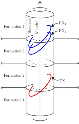
exploration usually employs LWD tools comprised of coil antennas wrapped around a metallic
mandrel inside a borehole, as illustrated in Fig. 1, a series of practical scenarios can be properly
approximate as a radially-stratified medium [6]. In this case, efficient algorithms based on
pseudo-analytical methods [6]–[10] are good alternatives to model these geometries and provide efficient
inversion algorithms designed to estimate the Earth formation properties given the tool responses.
More complicated geometries including inhomogeneities in the Earth formation along both radial and
axial directions can be accounted by using the numerical mode-matching (NMM), which may be seen
Pseudo-Analytical Modeling of
Tilted-Coil Antennas in
Anisotropic Geophysical Formations
Guilherme S. Rosa and José R. Bergmann,
Center for Telecommunications Studies, Pontifical Catholic University of Rio de Janeiro,
Rio de Janeiro, RJ 22451-900, Brazil, {guilhermesimondarosa, bergmann}@cetuc.puc-rio.br Fernando L. Teixeira
as providing a middle-ground in terms of computational costs between brute-force and
pseudo-analytical techniques [11]–[14]. The NMM is a very accurate approach that combines the FD or FE
method in one direction with an analytical (modal) expansion in the other directions.
Tilted-coil antennas (TCA) have been introduced for well-logging tools [7]–[9] to provide
azimuthal sensitivity. In [14], the NMM was extended to model triaxial TCA tools in vertical wells
with both radial and axial stratifications using a vertical mode expansion in conjunction with a horizontal mode-matching. The NMM can be also formulated in an alternate fashion, i.e., with a
horizontal mode expansion [10]–[13]. However, since TCA has a non-zero span along the axial direction, the vertical mode expansion is more appropriate to this type of problem. Although suitable
to model TCA tools in straight wells, the approach used in [14] cannot be easily generalized to curved
wells where axial bending is also present. These wells occur during deviated drilling and, in this case,
the axial (vertical) mode-matching is a more natural choice.
In this work, we employ an axial mode-matching combining attractive features of the early
described pseudo-analytical techniques, to obtain a flexible technique for analyzing directional
well-logging tools in anisotropic formations which can be easily extended to model wells with curvature.
II. PSEUDO-ANALYTICAL FORMULATION
The geometry shown in Fig. 1 is used to model different sections of the regions around the
well-logging tool as a bounded, radially-stratified waveguide. We can decompose the radiated field into
axial (to z) and transversal components, and the subscripts z and s, respectively, are used to assign
those directions. Our media is characterized by the complex permeability m = diag( ,m m ms s, z) and
permissibility = diag( , , s s z) tensors in cylindrical coordinates. Field solutions for Maxwell's
equations in uniaxially anisotropic multilayered cylindrical structures are well-known, and to avoid
repetition, we adopt here a notation similar to that in [2], [7], [9], [13]–[15] by assuming a
time-harmonic dependence in the form exp(-i tw ). A brief theoretical background of the formulation will
be presented in this section. More mathematical details can be found in [16].
A. Electromagnetic Fields Along Radial Stratifications
The forward propagating axial fields can be written in a compact fashion as
, , , 1 ( ) .
( ) z np
z z np in ik z
z n p z np
E e e H h f r r ¥ ¥ + =-¥ =
é ù é ù
ê ú = ê ú
ê ú ê ú
ë û
å å
ë û (1)The modal propagation constant in the z direction is kz np, , and the radial propagation constant kr,np
satisfies
2 2 2 2 2 ,np s z np, , s s s.
kr =k -k k = w m (2)
In order to simplify the notation, we will temporarily drop the modal subscript np and also the
argument of ez np, and hz np, , restoring them later as needed. The radially-dependent coefficients in (1)
are given by a linear combination of first kind Hankel and Bessel function of integer order n, as
given in [15], [16]. The transversal field components can be expressed as a combination of the axial
ones using well-known relations for cylindrical coordinates [13].
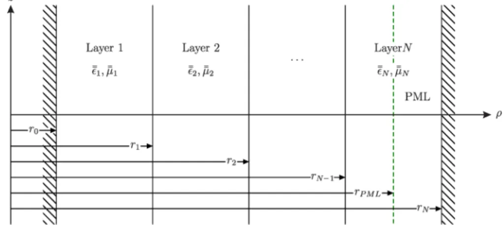
Consider the radially stratified waveguide shown in Fig. 2, composed by N layers. Each layer is
formed by an uniaxially anisotropic medium over rj-1 < <r rj, j =1, 2,¼,N , and for
0<f<2p. The fields at each layer j can be written, in a shorthand notation, as
or
, 1
( ) ( ) ,
j n j j n j j j j j
g a = éêHa k rr +Ja k r Rr + ùúa
ë û (3)
, 1
( ) ( ) ,
j n j j j j n j j j
g a = éêHa k r Rr - +Ja k rr ùúb
ë û (4)
where gja =[eja hja]t is a 2-by-1 column vector with the electric and magnetic non-harmonic
portion of the fields components in direction a={ , , }r f z . Notice that due the translational and
azimuthal invariance of the problem; see [13, pp. 163–164]; both z and f dependences can be
suppressed in (1). In order to enforce the appropriated boundary conditions at r =rj, we employ
by-2 generalized reflection matrices Rj j, 1 as in [13, Chap. 3], [15]. We can find the amplitudes of
adjacent layers to layer j using
and
1 , 1 , 1 , 1 ,
j j j j j j j j
a + =S +a b- =S -b (5)
where Sj j, 1 is defined in [13].
Using (5) in (3) and (4), it follows
, 1 , 1 , 1 , 1
(I -Rj j+Rj j- )bj =(I -Rj j-Rj j+ )aj = 0, (6)
which allow us to find the guidance condition for the modes as det(I -Rj j, +1Rj j, -1)=0. Since
, 1 , 1
N N N N
R + =R + [13], by setting M =I -RN N, +1RN N, -1, the eigenvalue solutions of
characteristic equation
det( )M = 0 (7)
are the discrete values of kz that contribute to our modal solution. We can next find all desired
eigensolutions of (7) in a given region of the complex plane kz (or kjr) using the Argument Principle
[17], [18] and the technique shown in [19].
Instead of matching the source jump condition to derive the eigenmode amplitudes as in [7], [9],
[14], here we prefer find a source-free solution and then include the excitation apart. We can easily
verify that solutions to the homogeneous linear system MbN = 0 correspond to the null space ofM ,
i.e., bN = null( )M . Now we have the modal amplitudes for the outermost radial standing wave, the
fields in all layers can be derived recursively using (5) and (4).
In order to mimic an unbounded medium, the radial direction is truncated by a perfectly matched
layer (PML) [20], [21]. The PML extends over rPML <r<rN, as illustrated in Fig. 2, and we use
the complex coordinate stretching formulation of the PML because it allow us to reuse all close-form
eigenmode formulas shown above, such we just need to select an appropriated complex-value for the
outermost radius of the waveguide [21]–[23], i.e., rN rN =rN +iaPML.
B. Electromagnetic Fields Along Axial Stratifications
The previous results can be applied to analyze an axially infinitely-long cylindrical waveguide. To
properly model the axial discontinuities shown in Fig. 1, we need to match the boundary condition at
each waveguide junction. Now, looking at equation (1), we can anticipate that the nth modal field of
region j will couple with only the (-n)th field of the adjacent regions j 1. This is due to the
orthogonality of the azimuthal harmonics and allows us to substantially simplify our analysis.
By imposing the conservation of reaction [24], [25] of the fields in the common aperture (at z =z1
in Fig. 3) between the regions 1 and 2, we can relate the forward and backward modal amplitudes in
each waveguide as
1 12 21 1 12 21 2 2
,
A R T A
T R
A A
- +
+
-é ù é ùé ù
ê ú = ê úê ú
ê ú êë úûê ú
where the generalized scattering matrix (GSM) comprises
1 1 1
12 ( 1 12t 2 12) ( 1 12t 2 12),
R = Q +X Q-X - Q -X Q- X (9)
1 1 21 2( 1 12t 2 12) 12t ,
T = Q +X Q- X - X (10)
and
1 1 12 2( 2 12 1 12t ) 12,
T = Q +X Q- X - X (11)
1 1 1
21 ( 2 12 1 12t ) ( 2 12 1 12t ).
R = -Q +X Q-X - Q -X Q- X (12)
The entries of matrices Q1, Q2 and X12 are closely related with the self-reaction of fields in region 1
and 2, and to the reaction of fields in region 1 to region 2, such as
12 p p, 1(np),2( np),
X ¢ = X - ¢ (13)
, ( ), ( )
, ,
j p p p p j np j np
Q ¢ = d ¢X - ¢ (14)
where dp p, ¢ denotes the Kronecker delta, and the reaction integrals are defined in terms of the fields in
regions i and j as
0
( ), ( ) 2 ( , , , , ) .
N
r
i np j np i np j np i np j np
r
X - ¢ = - p
ò
er h f ¢ +ef h r ¢ r rd
(15)
We are able to obtain analytical results for the above coupling integral as in [16], [22], [26].
The above procedure can be applied to all remaining axial discontinuities, allowing us to get one
GSM to each axial discontinuity.
C. Mode Excitation from a TCA Source
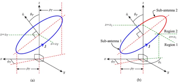
Consider a transmitter TCA with electrical current density given by
ˆ
( ) ( tan cos( ))( ˆtan sin( )),
T T T T T T T T
I d r r d z z r q f f f z q f f
= - - + - +
-J (16)
where IT is the current source amplitude, rT and zT are the radial and axial position of the coil, and
T
f and qT are the azimuthal and elevation tilt angles [7] as shown in Fig. 3 and Fig. 4a.
The electromagnetic field radiated by such transmitter TCA can be expressed in terms of the
waveguide modes as
, ( )
, ,
, 1
[ ( ) ˆ ( )] ikz np z zT in ,
s np z np
T np
n p
A r ze r e f
¥ ¥
- +
=-¥ =
=
å å
E e (17)
, ( )
, ,
, 1
[ ( ) ˆ ( )] ikz np z zT in ,
s np z np
T np
n p
A r zh r e f
¥ ¥
- +
=-¥ =
=
å å
+H h (18)
forz zT rT tanqT . By using the Lorentz reciprocity theorem [27, p. 41], we can determine the
unknown modal amplitude AT np, as
, , np T np np S A N
= (19)
where the source excitation
,
, ( ) (1 , ) , ( ) tan 2( , )
[
]
ikz np Tznp T T np T T z np T T T
S =I r ef r I - n k e r q I - n k e (20)
is normalized by Nnp = -2Xj np j( ), (-np). In the above, we consider that the source is inside the
region j, and the appropriated radial layer (of regionj) must be selected based on the value ofrT,
andkT = rT tanqT z npk , . Furthermore, I1 and I2 correspond to simple integrals over the azimuthal
angle given by
and
cos cos
1( , ) in i , 2( , ) sin in i ,
I n pe f k fd I n p e f k fd
p p
k + f k f + f
-
-=
ò
=ò
(21)which can be solved in closed-form [7]. As a further simplification, we can show that our initial series
solution in (17) and (18) reduces to a cosine series for positive integer n as shown in [16].
By combining the source amplitudes AT np, with the GSM matrices, the modal amplitudes AR np, can be obtained at an observation point on the plane z =zR, as shown in Fig. 3. After a few
simplifications, the receiver voltage (e.m.f.) can be obtained by performing a line integral of the
electric field along the receiver TCA.
Fig. 4. Tilted-coil antenna with electrical current density J completely inside one axial region is represented in (a).
In this analysis, we consider that the TCAs are completely inside one axial region. If that is not the
case, we can partition the TCA into segments associated to each region, calculate the contribution of
each segment individually, as suggested in representation shown in Fig. 4b, and use the superposition
to find the total radiated field. In this way, we must split the integration over f into (21) by means of
an appropriated value of fi as show in Fig. 4b. These integrals do not compute in closed-form but a
suitable fast convergent series representation exists based on the Jacobi-Anger expansion [28, p. 361].
III. NUMERICAL RESULTS
A. Validation
To illustrate the application of the proposed method, we present simulations of a triaxial logging
tool consisting of one transmitter and two receivers TCAs in a vertical-well borehole traversing an
anisotropic Earth formation with two horizontal layers. The problem includes a 4-in-radius metallic
mandrel, in which the TCAs are placed around, at the fixed radial distance rT R, = 4.5 in. We
consider a 5-in-radius borehole filled with oil-based mud having the isotropic conductivity
4
5 10
s = ´ - S/m. Surrounding the borehole, the horizontal and vertical component of the
conductivity of the bottom formation are 5 and 1 S/m. The top formation is characterized by 1 and
5 S/m, respectively. The axial positions of the transmitter, and receivers RX2 and RX1 (see Fig. 1)
are zT, zT +24 in and zT +30 in, respectively. This geometry was considered before in [2], [8]
and is used here to validate our formulation. For more details on this geometry, see [2], [8]. We
truncate the radial domain at 60 in, at about four times the skin depth of the les conductive layer. We
include all modes whose axial attenuation is less than 60 dB at 5 in, and have considered only
azimuthal indexes n = 0 and n =1. The high order azimuthal harmonics give negligible
contribution to total solution.
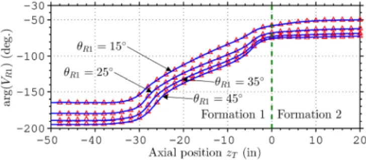
Fig. 5 and Fig. 8 plot the voltage due to a unit current excitation (IT =1 A at 2 MHz) at the
receivers antennas RX1 and RX2 as a function of the axial position zT of the tool, considering a
transmitter TCA with fixed tilt angle of 45, and four different receiver TCA tilt angles:
15 , 25 , 35
R
q = and 45. Very good agreement is observed versus the results from [2]
B. Modelling TCA Antennas inside Mandrel Grooves
After validating our new pseudo-analytical formulation, we now analyze the effect of a more
realistic source excitation. Instead of install the TCA antennas around the mandrel, we consider the
antennas now are wounded inside grooves on the mandrel pipe, as illustrated in Fig. 9. The mandrel
presents a radius of 4 in, and the indentations are 2-in-depth in radial direction. The TCA antennas
are placed at r= 3 in. The axial position of the antenna TX is on middle of a 8-in-groove, as shown
in Fig. 9. The receivers TCA antennas RX1 and RX2 are placed inside a 14-in-groove, such these receivers are 30-in and 24-in far from the transmitter. We consider a borehole filled with oil-based
mud having the isotropic conductivity s = ´5 10-4 S/m. The surrounding soil formation is an anisotropic media, and its horizontal and vertical component of the conductivity are 5 and 1 S/m,
respectively. Also, we consider that all antennas are azimuthally aligned, i.e., fT =fR1 =fR2.
Assuming a unit current excitation at 2 MHz, the tilt angle of each TCA antenna will be investigated
in the following. We truncate the radial domain at 60 in, and have include all modes whose axial
Fig. 6. Voltage phase at TCA receiver RX1. The results from the present approach are shown by solid lines. The small triangles are results from [2].
Fig. 7. Voltage amplitude at TCA receiver RX2. The results from the present approach are shown by solid lines. The small triangles are results from [2].
attenuation is less than 30 dB at 1 in; a very conservative criteria. Again, only azimuthal indexes
0
n = and 1 are included because the contribution of the high order ones are negligible.
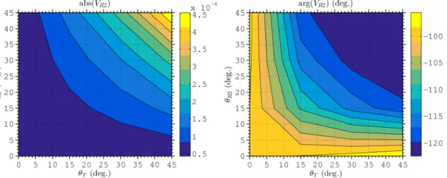
Fig. 10 shows results for the voltage at TCA receiver RX1 for various values of qT and qR1, in
which the tilt angles vary from 0 to 45. Similarly, Fig. 11 presents the voltage at RX2 for several
tilt angles associated to this receiver antenna. We can see that as the tilt angle of TCAs increases, the
received voltage becomes higher as well.
Fig. 9. Model employed to simulate the mandrel indentations. The details of the antennas positions and the dimensions
of grooves on mandrel are shown on the right, in which the TCAs have rT = rR1 = rR2 = 3 in.
In geophysical prospection using LWD tools, the parameters of interest are the amplitude ratio
(AR) and phase difference (PD) between the voltages at two antennas [2]:
,
10 2 1
20 log ( R / R )
AR = V V (22)
2 1
arg( R ) arg( R ).
PD = V - V (23)
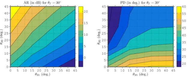
Proper combination of the results showed above in Fig. 10 and Fig. 11 allow us to describe AR and
PD responses for a desired LWD tool under investigation. Considering fixed transmitter TCA tilt
angles qT =0 , 15 , 30 and 45, we can derive the results shown in Fig. 12–Fig. 15.
For qT = 0, only fields associated to azimuthal order n =0 are excited, such AR and PD due
tilts in receivers observed in Fig. 12 cover the range of 8.4dB to9.8dB and 37 to46, respectively.
As said before, for qT >0, fields with n = 0 and n =1 represent the main contribute to received
voltage. In Fig. 13 we can clearly see the effects of fields with azimuthal index n =1 when
15
T
q = : now the variations of AR and PD are over 1dB to17dB and 23to55. This range of
variation increase with qT, as illustrated in Fig. 14 (for qT = 30) and Fig. 15 (for qT =45).
Notably, in these two cases we can observe negative values for AR; i.e, for some combinations of
1
R
q and qR2 the voltage received by RX1 is larger than those in RX2 (which is closer to TX).
Fig. 12. Amplitude ratio and phase difference response for a transmitter TCA with qT = 0 in respect to the tilt angle of receivers.
Fig. 13. Amplitude ratio and phase difference response for a transmitter TCA with qT = 15
in respect to the tilt angle of receivers.
Fig. 14. Amplitude ratio and phase difference response for a transmitter TCA with qT = 30
in respect to the tilt angle of receivers.
IV. CONCLUSION
We have introduced a new pseudo-analytical formulation to model tilted-coil antennas tools in
anisotropic formations. The combination of well-known closed-form solutions of Maxwell's equations
in cylindrical coordinates with an efficient PML allows us to express the fields in radially-layered
Earth formations as a sum of discrete modes. The TCA source is expanded in terms of modal fields,
and the fields are found using axial mode-matching. We showed numerical results to validate the
method and illustrate its ability to analyze directional well-logging tools. As a future work, this
technique will be extended to analyze the fields in curved wells.
ACKNOWLEDGMENT
The first author acknowledges support from the Brazilian Agencies CNPq and CAPES through the
doctoral fellowships 140236/2013-9, 141847/2016-6 and 000316/2015-06.
REFERENCES
[1] Y.-K. Hue and F. Teixeira, “FDTD simulation of MWD electromagnetic tools in large-contrast geophysical formations,” IEEE Trans. Magn., vol. 40, pp. 1456–1459, Mar. 2004.
[2] Y.-K. Hue, “Analysis of electromagnetic well-logging tools,” Ph.D. dissertation, The Ohio State University, Columbus, 2006.
[3] H. O. Lee and F. L. Teixeira, “Cylindrical FDTD analysis of LWD tools through anisotropic dipping-layered earth media,” IEEE Trans. Geosci. Remote Sens., vol. 45, pp. 383–388, 2007.
[4] M. S. Novo, L. C. da Silva, and F. L. Teixeira, “Three-dimensional finite-volume analysis of directional resistivity logging sensors,” IEEE Trans. Geosci. Remote Sens., vol. 48, no. 3, pp. 1151–1158, Mar. 2010.
[5] ——, “A comparative analysis of krylov solvers for three-dimensional simulations of borehole sensors,” IEEE Geosci. Remote Sens. Lett.,vol. 8, no. 1, pp. 98–102, Jan. 2011.
[6] J. Lovell and W. Chew, “Response of a point source in a multicylindrically layered medium,” IEEE Trans. Geosci. Remote Sens., vol. 25, pp. 850–858, Nov. 1987.
[7] T. Hagiwara et al., “Effects of mandrel, borehole, and invasion for tilt-coil antennas,” in SPE 78th Ann. Tech. Conf. Exhibit., 5–8 Oct. 2003.
[8] Y.-K. Hue and F. L. Teixeira, “Analysis of tilted-coil eccentric borehole antennas in cylindrical multilayered formations for well-logging applications,” IEEE Trans. Ant. Prop., vol. 54, pp. 1058–1064, 2006.
[9] G. S. Liu, F. L. Teixeira, and G. J. Zhang, “Analysis of directional logging tools in anisotropic and multieccentric cylindrically-layered earth formations,” IEEE Trans. Antennas Propag., vol. 60, pp. 318–327, Jan. 2012.
[10]H. Wang, P. So, S. Yang, W. J. R. Hoefer, and H. Du, “Numerical modeling of multicomponent induction well-logging tools in the cylindrically stratified anisotropic media,” IEEE Trans. Geosci. Remote Sens., vol. 46, no. 4, pp. 1134– 1147, Apr. 2008.
[11]W. C. Chew et al., “Diffraction of axisymmetric waves in a borehole by bed boundary discontinuities,” Geophys., vol. 49, pp. 1586–1595, 1984.
[12]Q.-H. Liu, “Electromagnetic field generated by an off-axis source in a cylindrically layered medium with an arbitrary number of horizontal discontinuities,” Geophys., vol. 58, pp. 616–625, 1993.
[13]W. C. Chew, Waves and Fields in Inhomogeneous Media. New York, NY: IEEE Press, 1995.
[14]Y.-K. Hue and F. Teixeira, “Numerical mode-matching method for tilted-coil antennas in cylindrically layered anisotropic media with multiple horizontal beds,” IEEE Trans. Geosci. Remote Sens., vol. 45, pp. 2451–2462, 2007. [15]H. Moon, B. Donderici, F. L. Teixeira, “Stable evaluation of Green's functions in cylindrically stratified regions with
uniaxial anisotropic layers,” J. Comp. Phys., vol. 325, pp. 174–200, 2016.
[16]G. S. Rosa, J. R. Bergmann, and F. L. Teixeira, “A robust mode-matching algorithm for the analysis of triaxial well-logging tools in anisotropic geophysical formations,” IEEE Trans. Geosci Remote Sens., submitted, 2016.
[17]L. M. Delves and J. N. Lyness, “A numerical method for locating the zeros of an analytic function,” Mathematics of Computation, vol. 21, no. 100, pp. 543–560, Oct. 1967.
[18]J. W. Brown and R. V. Churchill, Complex Variables and Applications, 7th ed. New York, NY, USA: McGrawHill, 2004.
[19]G. S. Rosa and J. R. Bergmann, “Pseudo-analytical modeling for the electromagnetic propagation in stratified cylindrical structures,” IEEE Antennas Wireless Propag. Lett., vol. 15, pp. 344–347, 2016.
[20]W. C. Chew and W. H. Weedon, “A 3D perfectly matched medium from modified Maxwell’s equations with stretched coordinates,” Microw. Opt. Tech. Lett., vol. 7, pp. 599–604, 1994.
[21] F. L. Teixeira and W. C. Chew, “Complex space approach to perfectly matched layers: a review and some new developments,” Int. J. Num. Model., vol. 13, pp. 441–455, 2000.
[23]P. Bienstman and R. Baets, “Advanced boundary conditions for eigenmode expansion models,” Optical and Quantum Electronics, vol. 34, no. 5, pp. 523–540, May. 2002.
[24]R. F. Harrington, Time-harmonic electromagnetic fields. New York, NY, USA: McGraw-Hill, 1961. [25]V. H. Rumsey, “Reaction concept in electromagnetic theory,” Phys. Rev., vol. 94, pp. 1483–1491, Jun. 1954.
[26]K. Zaki, S.-W. Chen, and C. Chen, “Modeling discontinuities in dielectric-loaded waveguides,” IEEE Trans. Microw. Theory Techn., vol. 36, no. 12, pp. 1804–1810, Dec. 1988.
[27]D. M. Pozar, Microwave Engineering, 3rd ed. Hoboken, NJ, USA: John Wiley & Sons, Inc., 2005.