Abstract It is shown that proper representation of transmitting and receiving antennas in indoor environments are decisive for accurate prediction of electromagnetic power transfer parameters using the standard 3D-FDTD method. With the standard Yee method, it is not always possible to precisely describe all the geometrical details of electrically small antennas. A new approach for description of the discone antenna in uniform 3D-FDTD lattice is presented. The calculations are validated by comparing FDTD results with the polyhedral beam-tracing method and experimental data.
Index Terms— Channel characterization, power delay profile, 3D-FDTD, electrically small antennas, large computational environments.
I. INTRODUCTION
For designing communication systems, the electromagnetic characteristics of communication
channel must be trustworthily known [1]. With computational simulations [2], it is possible, for
example, to determine the optimal position of the transmitting antenna to maximize the coverage area
and to identify multipath phenomena calculating the power delay profile (PDP). This parameter can
be calculated using the procedure given in [1,3], which avoids the use of deconvolution algorithms to
obtain impulsive responses of the channel.
Based on the discone antenna in [4] which is electrically small, a new antenna was designed, built
and used in the measurements presented in [3,5]. Its straightforward numerical representation in such
electrically large indoor environments is limited by computational restrictions when the standard 3D
finite-difference time-domain (3D-FDTD) method [2] is used, even when a powerful computer cluster
is used. It means that an extremely high number of Yee cells [2,6] would be required for modeling
the entire environment containing the antenna if a globally uniform grid is used. Alternative solutions
would be using locally non-orthogonal or locally refined orthogonal grids [2,6], which can be,
respectively, mathematically intricate [7] or numerically demanding because stability is usually
achieved using considerably small time steps [2].
In this paper we introduce an equivalent FDTD representation of the discone antenna, which is
used as transmitter and receiver, in such a way that most of its characteristics (polarization, operating
frequency band and radiation patterns) are approximated using a globally coarse grid, thus preserving
Indoor Characterization of Power Delay
Profile Using Equivalent Antenna
Representation in Uniform FDTD Lattices
Bruno W. Martins, Rodrigo M. S. de Oliveira, Victor Dmitriev, Fabrício J. B. Barros and Nilton R. N. M. Rodrigues.
Federal University of Pará, Belém-PA, Brazil
the simplicity, elegance and the original efficiency of Yee method. In addition, the introduced
procedure significantly simplifies computer implementation because complications inherent to
non-uniform or non-orthogonal grids are circumvented [2, 6]. With the proposed approach, the obtained
numerical results characterizing the indoor environment become much closer to the experimental data
than the numerical results presented earlier in [3].
II. MEASUREMENT ENVIRONMENT
A. Indoor environment
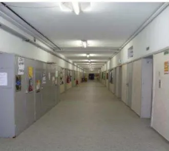
In Fig. 1, we show the indoor environment used for performing experimental and numerical
analyses of time spread parameters of electromagnetic signals. It is a corridor on the second floor of
the building Cardeal LEME at PUC-Rio university. During experiments, a vector network analyzer
was used as a transceiver exciting 1601 sinusoidal carriers uniformly separated by approximately 0.53
MHz in the frequency band ranging from 950 MHz to 1800 MHz, as presented in [3,5]. A descriptive
list of the parameters of the measurements is given in Table I.
Fig. 1. Corridor of field measurements: this environment is reproduced numerically using the 3D-FDTD Method.
TABLE I. MEASUREMENT SETUP PARAMETERS [3,5]
Parameters Values Frequency range
Bandwidth Number of samples Time resolution (∆�) Maximum delay Analysis time
Frequency spacing between samples Transmission power
Amplifier gain
Cable and connector losses
950 to 1800 MHz 850 MHz 1601 1.17 ns 1882.35 ns 346 ns 0.53 MHz 10 dBm 25 dB 5dB
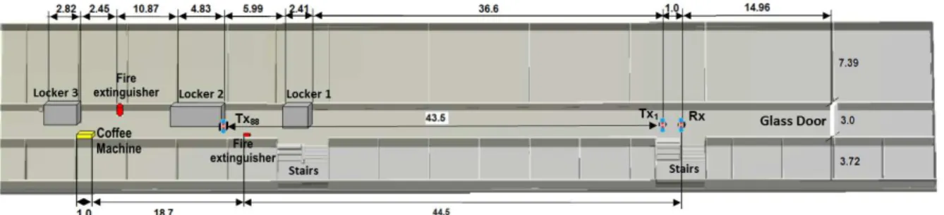
Fig. 2 shows the floor plan of the indoor environment of Fig. 1. During measurements, there were
transmitting and receiving antennas have been positioned at the height of 1.5 m above the floor for
performing LOS (line-of-sight) propagation analysis. The transmitter was positioned at 88 different
points, being moved away from the receiver 0.5 m each time in straight line in the corridor, as
indicated by Fig. 2. The first position of the transmitter Tx1 is one meter away from the receiver Rx
and the last position analyzed Tx88 is 44.5 m away from Rx. Notice that the used time to obtain the
amplitudes and phases is 1.882 µs for each position of the transmitter.
B. Numerical modeling of environment
In our computer representation of the environment defined by the floor plan in Fig. 2, most objects
were modelled for signal prediction. Electrically small objects, as the fire extinguisher and the coffee
machine, are also considered in our numerical FDTD model. In Table II, the dimensions and
electromagnetic characteristics (relative permittivity �� and conductivity σ) of each object considered
in the simulation can be seen. The FDTD representation of the environment was developed using the
software SAGS [8]. The polyhedral beam-tracing model follows [3,9]. For the FDTD model, the
parameters in Table II were set individually for each field component in Yee’s cells to properly define
each dielectric or conducting block forming the indoor scenario. The discretization is uniform
throughout the environment and it is based on cubic Yee cells with 3 cm-long edges (=3cm). The
total FDTD mesh size is 3120×520×175 and the time step was set to 99% of Courant’s limit [2]. FDTD and PBT models were applied to the environment shown in Fig. 2 with the parameters of Table
II.
Fig. 2 SAGS 3D-view of the FDTD model of LEME, with position markers of transmitter (Tx1 and Tx88) and receiver (Rx);
all dimensions are given in meters.
TABLE II. PHYSICAL PARAMETERS OF OBJECTS CONSIDERED IN FDTD AND PBT MODELS
Object Material Dimensions (m) εr σ (S/m) μr
III. THE PROPOSED EQUIVALENT FDTD REPRESENTATION OF THE DISCONE ANTENNA
The antenna used in the measurements is a discone antenna illustrated by Figs. 3(a) and 3(b). For
the frequency range 950-1800 MHz, its gain as a function of the elevation angle θ is shown in Fig.4.
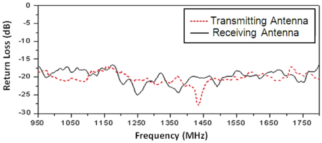
The return loss of the discone antenna is approximately constant under -15 dB, as shown by Fig. 5.
The discone antenna has an omnidirectional radiation pattern and return loss below -15 dB in
frequency range of interest, as shown by Figs. 4 and 5, respectively.
As previously discussed, there are issues for representing computationally the discone antenna
geometry of Fig.3(a) using the standard 3D-FDTD method for the electrically large problem. Thus, an
equivalent representation of the antenna is suggested for modeling the device in uniform FDTD
lattices (Fig. 3c).
(a) (b) (c)
Fig. 3. Discone antenna: (a) schematics, (b) photograph of the constructed antenna used in experiments and (c) optimized equivalent antenna for FDTD simulations.
Fig. 5. Measured return losses of discone antennas.
For the maximum frequency considered (1.8 GHz, Fig.5), we have a wavelength of approximately
16.66 cm. We see in Fig. 3 that the total height of the antenna is 15.6 cm, which is smaller than the
minimum wavelength considered. All other dimensions of geometric details are even smaller. For the
lower frequencies considered (Fig. 5), the electric lengths of the constituent parts of the discone
antenna are even less significant. Due to the large electrical length of the indoor environment, we
have used =3cm. Local refinements of FDTD discretization over the antenna could be used for
representing the small features of the device, but this would force substantial reduction of the time
step t (which must be avoided) [2]. Although the minor geometric details are not extremely
important (for the considered electric lengths), larger details must be geometrically approximated in
order to produce properly approximated radiation patterns. That is why the proposed model has the
shape shown in Fig.3(c). However, because =3cm, this representation is larger than the original
antenna. Thus, in order to reduce its electric length, capacitors have been used for compensating for
the reactive impedance, which is inductive. Clearly, the antenna polarization is preserved in the
equivalent model.
To compare the equivalent representation and the real discone antenna, we have calculated the
return loss RL given by
�� = − . log |� − �� + ���|. (1)
In (1), ZSis the load impedance (50 Ω) and Z is the impedance of the simulated antenna obtained
through point-by-point division of the Fourier transforms of voltage � � and current � in a
discrete frequency spectrum. Mathematically, one has
� � =ℱ{� � } .ℱ{ � } (2)
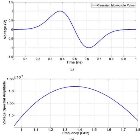
The voltage V(t) is the excitation pulse, which is a function of time t (Fig. 6(a)). The voltage is
antenna (Fig. 3(c)). The source is implemented by setting Ez source
= V(t)/, where is the FDTD spatial
increment (cubic Yee cell edge length). The pulse V(t) is a Gaussian monocycle function (time
derivative of a Gaussian pulse) given by
� � = ��(� − . �� ) exp [− (� − . �� ) ], (3)
where ��= and � = . 8 × − s are the pulse amplitude and width, respectively. As it can
be seen in Fig. 6(a), the pulse has duration of approximately 0.85 ns. The frequency range of the
excitation signal in Fig. 6(b) contains significant power in appropriate frequency band between 950
MHz and 1800 MHz. The current is calculated in one of the antenna rods, in the cell neighboring the
electric field excitation cell (antenna’s gap), by evaluating the curl of magnetic field around the
cylindrical rod, which is multiplied by the area of the face of secondary Yee’s cell [2] orthogonal to
the referred rod.
With this data, it is possible to determine the return loss of the preliminary dipole antenna. The
antenna return loss is below –2 dB (black solid line) in the desired frequency range, as shown by Fig.
7(a). This value is above the value produced and measured for the real antenna. Thus, adjustments for
this preliminary antenna are important for providing a return loss profile similar to those shown by
Fig. 5.
(a)
(b)
It is known, from physics, that reducing the length of the antenna would displace the return loss
point of minimum to a higher frequency, as required. However, this adjustment would also lead to
very small Yee cells in classic FDTD method, increasing computational demands. Furthermore, local
grid refinements (around the antennas) would impose the use of exceedingly small time steps [2].
Numerous tests were conducted considering adjustments to the model proposed. The goals are to
make the simulated antenna to provide a return loss profile under ̶ 4 dB or ̶ 6 dB (as it is expected for indoor applications [10-13] and to approximate the gain of the equivalent antenna to the gain of the
antenna used in experiments. For this purpose, the model shown in Fig. 3(c) is proposed. For
representing the metallic parts indicated in Figs. 3(a) and 3(b), we have included cubic metallic blocks
in the equivalent model illustrated by Fig. 3(c). Two syntonizing capacitors, modelled using the
technique described in [14], are incorporated between the rods and the metallic blocks, as shown by
Fig. 3 (c). The idea is to tune the antenna with the band of interest, i.e., to provide the impedance
matching between the rods and the metallic block. In order to achieve the results shown in Fig. 7,
other parameters were adjusted along with the syntonizing capacitance C, namely the lengths and
radius of the rods. Increasing the radius r of the rods contributes positively to reduce the return loss
values (dotted lines in Fig. 7(a)). The highest value used for the radius of the rod, which provides
precision of the simulations and minimizes the return loss, is 12.65 mm.
The antenna used in the experiments is 15.6 mm in length (Fig. 3 (a)). However, the spatial step of
the FDTD lattice was set to 3 cm due to computational restrictions imposed by the indoor
environment. Thus, the equivalent model has a length of 21 cm as shown by Fig. 3 (c) and, for this
reason, the capacitors are also necessary for reducing the electrical length of the model, as it is
illustrated in Fig. 7(a).
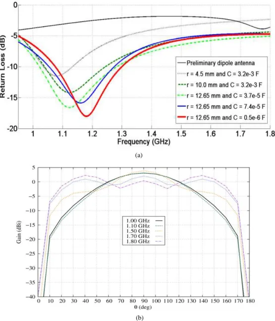
The solid lines in Fig.7(a) show that the return losses obtained with the capacitors of 0.5µF are
closer to experimental curve of Fig. 5 for 1.05 GHz ≤ f ≤ 1.30 GHz than the return losses
calculated for the preliminary dipole antenna (with no capacitors). For this reason, the value of the
(a)
(b)
Fig. 7. Parameters of proposed antenna: (a) return losses for various capacitances and (b) gain obtained with capacitors of 0.5µF.
The modeled antenna provides return losses of less than –10 dB, for approximately 35% of the
frequency range of interest, as it can be seen in Fig. 7(a). For broadband antennas, it is suggested in
[9] to consider the value of – 6 dB as a threshold in the study of return loss in the frequency range
considered. The suggested antenna has 83% return loss below – 6 dB. In addition, the entire return
loss profile is under –4 dB for the band of interest [12][13].
Finally, by comparing Figs. 4 and 7(b), it can be seen that the gain obtained using syntonizing
capacitors of 0.5 µF for the proposed antennas agree well with those obtained for the discone antenna
in [3]. We see that for 1 GHz and 1.1 GHz, the approximately omnidirectional profile is preserved by
the equivalent model. Also, for 1.5, 1.7 and 1.8 GHz, the oscillations seen in gain profiles of Fig. 4 are
IV. SIMULATION AND EXPERIMENTAL RESULTS
For simulations of the environment depicted by Fig. 2 with the 3D-FDTD method, more than
32 GB of RAM were necessary. The used computer system is a Beowulf cluster [15] based on a
distributed parallel architecture and on the message passing interface specification (LAM/MPI
Library). The technical specifications of each of the 16 cluster nodes are: processor Intel Core i5-3330
working at 3.0 GHz with 8 GB of RAM. The physical communication between the computers is
performed via a 16-port-switch with transfer rate of 1000 Mbps. The operating system used is the
Slackware Linux 64 bits, release 14.0. The processing time of 3D-FDTD simulation was
approximately six hours. An exact antenna representation has not been considered in this paper for
FDTD simulations. One of the motives is that the antenna is electrically small. Numerically, locally
non-orthogonal or locally refined orthogonal grids [2,14] could be used for representing the antenna.
However, the use of non-uniform FDTD lattices with very small cells would require a much larger
simulation time than the processing time necessary to conclude the FDTD simulation with the
equivalent antenna representation proposed in this work. This is mainly due to the mandatory
significant reduction of time step [2].
In order to validate the proposed FDTD equivalent antenna representation, and because it is
not possible to resolve problems modeled with 3D-FDTD without using a radiator as well as it is not
feasible to model an isotropic source [2], we used the polyhedral beam-tracing method (PBT), which
was previously validated in [3] with excitation by an isotropic radiator. PBT is a frequency domain
method, which is described in [3,9]. The PBT model ran on a notebook equipped with a 2.0 GHz
Intel Core 2 Duo processor with 1.0 GB of RAM. The Windows 7.0 operating system was employed.
The processing time was 44.2 and 42.1 minutes for simulations with non-isotropic and isotropic
antennas, respectively. The higher FDTD processing time compared to PBT is expected since in
FDTD one needs to discretize the entire environment using electrically small Yee cells. In addition,
all the six field components are calculated in each Yee cell for every discrete advance in time.
A. Analysis of the measured data
According to the configuration of the measurement campaign described in Section II, amplitudes
and phases of the signals were obtained for several points in the frequency band of interest (950-
1800MHz). These values are used to calculate the power delay profile [1] at the transceiver positions
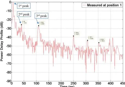
(Fig. 2). The power delay profile measured at the first position (receiver Rx positioned one meter
away from the transmitter Tx) is shown in Fig. 8 and displays several reflection peaks. These peaks
can provide locations of specific objects in scenario. Locations can be determined by estimating the
time that the signal needs to propagate from the transmitter to a reflecting object and finally arrive at
Fig. 8. Power delay profile measured at Tx1. Transmitter is 1 meter away from receiver.
Therefore, one can relate the time at which a peak is observed to walls and other objects in the
environment shown in Fig. 2. In Fig. 8, the first peak is due to direct wave incidence (the signal
propagates directly from the transmitter to the receiver). The second peak arrival time at the receiver
was observed to be 40 ns. This time defines a total propagating distance of 11.96 m. This distance is
likely to be associated with signal reflected in the stairs which are on the left side of the receiver
(Fig.2). Finally, in Table III we have estimated associations of the other peaks of the signal shown in
Fig. 8 with the scattering objects in the environment.
TABLE III ESTIMATED ASSOCIATIONS BETWEEN PEAK TIMES AND DISTANCES TO SCATTERING OBJECTS
Peak Time (ns) Total Propagation
Path (m) Object
17.65 40.00 109.4 250.6 307.1 352.9
5.28 11.96
32.7 74.93 91.82 105.52
Corridor wall Stairs 1
Wall with glass door Cabinet 1
Cabinet 2 Cabinet 3
B. Simulation results
In order to obtain the time domain power delay profile from transient FDTD signals, it is necessary
to implement a frequency-domain deconvolution algorithm to process the received signal.
Specifically, calculations are partially performed in frequency domain (using Fourier transforms) for
determining the channel transfer function � from the time domain voltages obtained between the
terminals of the transmitter (Fig.3) and between the terminals of the receiving antenna. The voltages
were calculated across the respective antennas’ gaps.
The propagation channel is considered to be purely linear. It can be thought as a linear system with
the transfer function H(f). Consequently, the Fourier transform Vi(f) of the transmitter voltage shown
by Fig. 6(b) is the input of the linear system. The output signal Vox(f) is the Fourier transform of the
The transient input and output voltages, obtained via FDTD method, are converted to the frequency
domain using the Filon integration method [16]. The discrete spectral values of the voltages thus
obtained are point-by-point divided for obtaining a discrete version of the channel transfer function � . Afterwards, one proceeds with the calculation of the impulse response ℎ � of the channel using ℎ � = ℱ− { � }, where ℱ− indicates the discrete inverse Fourier transform. The power
delay profile is defined in decibels as ��� = log |ℎ � |.
Since the return loss is a measure of the quantity of power returning to the source, we can say that,
with an adequate interpretation, it can indicate the amount of the power radiated by the antenna in a
given frequency (considering Joule effect negligible). In addition, because the indoor environment can
be considered as a linear system, from the physical point of view, it is easy to see that the amount of
power radiated by the antenna for a given frequency is, in fact, not important for obtaining H(f) and
consequently not important to define PDP. However, from the numerical point of view, if the
amplitudes of the fields at a given frequency are too low at the receiver, rounding errors on numerical
evaluations can produce incorrect values for H(f). For this reason, the return loss of the equivalent
transmitting antenna must be under -4 dB for the entire band of interest for ensuring that the signal
reaches the receiver with appreciable amplitudes in order to avoid rounding problems. This also
means that obtaining a specific profile of the return loss is not essential because H(f) is a relative
quantity.
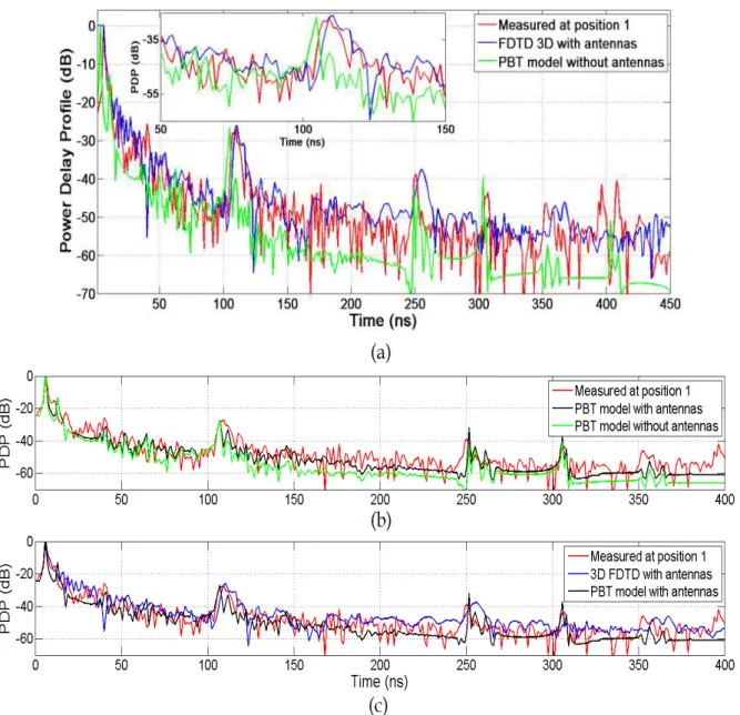
For the point Tx1 in Fig. 2, the results obtained using the 3D-FDTD and PBT methods are
compared with the experimental curve for power delay profile in Fig. 9. It can be seen in this figure
that when the proposed antenna model is used in the receiver at Rx1, the FDTD method can reproduce
most of the peaks shown in Fig. 8. The layout of the environment directly affects the amplitude and
position of the peaks obtained in the simulation. When the receiving antenna was removed, certain
peaks were inappropriately amplified (e.g. between 50 and 100 ns) and other were also improperly
attenuated (e.g. in the interval between 275 and 300 ns). This is strongly related to the radiation
pattern of the modeled receiving antenna, which is similar to the radiation profile of the discone
antenna, as one can see in Figs. 4 and 7(b). For the PBT results without antenna (Fig. 9b), we see that
some peaks are reproduced properly. However, for t > 50 ns, power delay profile is below the
experimental and FDTD curves. The average amplitude displacement is approximately –10 dB. This
is explained by the fact that the transmitting and receiving antennas were not considered in the present
PBT model simulation, differently from that performed in [3]. Consequently, each ray that goes out
from the transmitter in different directions (or arriving at the receiver) endures a 0dbi gain for all
frequencies and directions. When the transmitting antenna is absent, PBT results are equivalent to
those produced by using an isotropic radiator. However, when the antennas gain is considered in PBT
(Figs. 9b and 9c), the PDP amplitudes behave as if they were the moving average values of the
simultaneously included. Observe that performing 3D-FDTD simulations without antennas is not
possible [2]. It is worth to notice that for Fig. 10, in which results are obtained 44.5 m away from the
transmitter, PBT results present deviations similar to those seen in Fig. 9 (acquired 1 m from
transmitter).
For 3D-FDTD simulation, the multipath amplitudes in Figs. 9 and 10 present similar oscillating
behavior as in the measurement, especially for the delay values higher than 150 ns. The PBT power
delay profiles is relatively smooth, in comparison with the corresponding FDTD PDPs, since the
PBT model consider up to 11 interactions (reflections or transmission) with the environment [3].
Therefore, multipath amplitudes were not detected due to the limited rays interaction with the
environment’s objects.
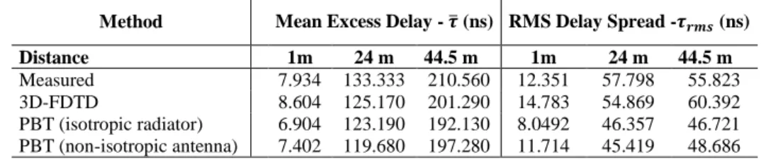
The simulated and measured parameters of the temporal fading are shown in Table IV for distances
1.0, 24.0 and 44.5 meters between transmitter and receiver. By analyzing PBT results, we see that the
inclusion of the antenna radiation characteristics improve results over PBT calculations which are
performed by using the isotropic radiator. However, numerical solutions obtained with 3D-FDTD
employing the proposed equivalent antenna representation are in much better accordance to the
measured data, validating the proposed methodology. Although a small part of the peaks are not
present in FDTD results, the arrival time of significant multipath components are very similar to the
experimental signal. The temporal fading of the channel was obtained considering the threshold of –
50 dB for Excess Delay Spread.
TABLE IV TIME SPREAD OF THE CHANNEL
Method Mean Excess Delay - �̅ (ns) RMS Delay Spread -�� (ns)
Distance 1m 24 m 44.5 m 1m 24 m 44.5 m
Measured 7.934 133.333 210.560 12.351 57.798 55.823 3D-FDTD 8.604 125.170 201.290 14.783 54.869 60.392 PBT (isotropic radiator) 6.904 123.190 192.130 8.0492 46.357 46.721 PBT (non-isotropic antenna) 7.402 119.680 197.280 11.714 45.419 48.686
PBT results in Figs. 9 and 10 lead to interesting conclusions regarding the impacts of the
shape of the equivalent antenna used in FDTD method. With PBT, we can model an isotropic source
[9]. Of course, radiation level is considered to be identical in every direction and for every frequency
considered (specifically, electric field is considered to always have unitary amplitude). The
transmitter is transparent: when electromagnetic field reflects in an object and returns to the source,
the field unimpededly goes through it. For the case in which a more realistic antenna is considered in
PBT, radiation levels are corrected for each direction and for each frequency. However, the antenna
itself is also considered to be transparent [9]. In these PBT cases, even when the transparent antenna
model is employed (which is evidently not the case of experiments), we see in Figs. 9 and 10 and in
the reflected signals (in the transmitting antenna) are of small amplitudes and thus have influence
mainly on low amplitude portions of the PDP signals. This means that radiation pattern is of more
importance than considering the exact shape of the antenna. This explanation justifies the fact that
FDTD results, obtained with the proposed equivalent antenna model, are in very good accordance
with experimental results: the radiation characteristics obtained with the model are compatible with
those obtained experimentally (Fig. 7). As previously discussed and predicted, radiation
characteristics are more important than representing in details the shape of the antenna for this kind of
problem. The equivalent antenna model cannot be electrically very large, otherwise reflections can be
appreciable and substantially modify the results and radiation characteristics can be drastically
affected
.
Fig. 9. Normalized PDP ̶ transmitter is placed 1 m away from receiver: (a) experimental, FDTD and PBT results with isotropic radiator (insert: PDP for time period between 50 and 150 ns), (b) experimental and PBT results with isotropic and
Fig.10. Normalized PDP ̶ transmitter is placed 44.5 m away from receiver: (a) experimental, FDTD and PBT results with isotropic radiator (insert: PDP for time period between 300 and 350 ns), (b) experimental and PBT results with isotropic and
non-isotropic radiators and (c) experimental, FDTD and PBT results with non-isotropic radiator.
V. CONCLUSIONS
In this paper, indoor power delay profile is calculated using the classic FDTD method. In order to
minimize processing time and the computational requirements for simulating the electrically large
indoor environment analyzed, a coarse uniform FDTD grid is employed. Experiments were performed
using a discone antenna. This antenna has electrically small geometric features, which cannot be
represented with the coarse FDTD lattice. It is shown that, for this kind of numerical analysis,
characteristics of the device used in experiments. In this context, an equivalent model is proposed for
the discone antenna. Numerical tests performed with the suggested representation were exceptionally
successful: FDTD results are in very good accordance with experiments, validating the equivalent
FDTD model developed for the discone antenna.
ACKNOWLEDGMENTS
This work was partially supported by CAPES via the RH-TV Digital project. Authors acknowledge the support received from researchers of PUC-Rio, especially professors Glaucio L. Siqueira, José R. Bergmann and Emanoel Costa. The first researcher, professor Siqueira, the master's degree advisor of Fabrício Barros (the fourth author of the paper), provided valuable support for executing the experimental measurements. Professor Bergmann also provided important insights for performing measurements. Finally, prof. Costa (PhD advisor of F. Barros) granted relevant technical discussions necessary for development of the PBT model.
REFERENCES
[1] H. Hashemi, “The Indoor Radio Propagation Channel”, Proceedings of the IEEE, vol. 81, pp. 943–968, 1993.
[2] A. Taflove and S. C. Hagness, Computational Electrodynamics, The Finite-Difference Time-Domain Method. Artech House Inc., 2005.
[3] F. J. B. Barros, E. Costa, G. L. Siqueira and J. R. Bergmann, “A polyhedral beam-tracing method for modeling
ultrawideband indoor radio propagation”, Microwave and Optical Technology Letters, vol.54, pp. 904-909, 2012. [4] J. R. Bergman, On the design of broad band omnidirectional compact antennas. IEEE Microwave and Optical
Technology Letters, vol. 39, pp. 418-422, October 2003.
[5] F. J. B. Barros, R. D. Vieira and G. L. Siqueira, "Relationship between delay spread and coherence bandwidth for UWB transmission," SBMO/IEEE MTT-S International Conference on Microwave and Optoelectronics, pp. 415-420, 2005.
[6] U. S. Inan and R. A. Marshall, Numerical Electromagnetics: the FDTD Method. Cambridge University Press, 2011.
[7] R. M. S. de Oliveira, and C. Sobrinho, “UPML Formulation for Truncating Conductive Media in Curvilinear
Coordinates”, Numerical Algorithms, vol. 46, pp. 295-319, 2007.
[8] R. M. S. de Oliveira and C. Sobrinho, “Computational environment for simulating lightning strokes in a power substation by finite-difference time-domain method”, IEEE Transactions on Electromagnetic Compatibility, vol. 51, pp. 995-1000, 2009.
[9] F. J. B. Barros, E. Costa, G. L. Siqueira and J. R. Bergmann, “A Site-Specific Beam Tracing Model of the UWB Indoor
Radio Propagation Channel”, IEEE Transactions on Antennas and Propagation, vol. 63,pp.3681-3694, 2015. [10]H. Karl and A. Willig, Protocols and Architectures for Wireless Sensor Networks, John Wiley & Sons, 2007.
[11]T. K. Sarkar, M. C. Wicks, M. S.-Palma and R. J. Bonneau, “Smart Antennas”, John Wiley & Sons, 2003.
[12]I. Henning, M. Adams, Y. Sun, D. Moodie, D. Rogers, P. Cannard, S. Dosanjh, M. Skuse, and R. Firth, “Broadband antenna-integrated, edge-coupled photomixers for tuneable terahertz sources,” IEEE Journal of Quantum Electronics, vol. 46, pp. 1498–1505, 2010.
[13]Z. Chen, Y. L. Ban, J. H. Chen, J. L. W. Li and Y. J. Wu, “Bandwidth Enhancement of LTE/WWAN Printed Mobile
Phone Antenna Using Slotted Ground Structure”. Progress In Electromagnetics Research, vol. 129, pp. 469-483, 2012. [14]T. Noda, A. Tatematsu and S. Yokoyama, Improvements of an FDTD-Based Surge Simulation Code and its
Application to the Lightning Overvoltage Calculation of a Transmission Tower, Electric Power Systems Research, vol. 77, pp. 1495-1500, 2007.
[15]D. J. Becker, T. Sterling, D. Savarese, J. E. Dorband, U. A. Ranawake and C. V. Packer, "BEOWULF: A parallel workstation for scientific computation", in Proceedings of International Conference on Parallel Processing, vol. 95, pp. 1-4, 1995.
![Fig. 4. The Gain of the discone antenna used in PBT model of [9], calculated for several frequencies using method of moments (MoM)](https://thumb-eu.123doks.com/thumbv2/123dok_br/18888460.424399/4.892.209.683.827.1102/gain-discone-antenna-model-calculated-frequencies-method-moments.webp)