Abstract— This paper addresses the impact of magnetization level tolerances in ferrite-based permanent magnets (PM) on the performance of brushless DC motors. A case study is prepared using three motor prototypes assembled with controlled samples of ferrite arc segments, in terms of magnetization. The investigation is performed both experimentally and through simulations using the software SPEED. The results show that narrow tolerance margins for the magnetization conditions in the production line can potentially minimize the use of raw material on such motors whereas keeping the efficiency and torque behavior required by the application.
Index Terms—brushless DC motors; machine testing; magnetization; ferrite magnets; quality assurance; quality control; magnetization quality assessment.
I. THEDEPENDENCEOFMOTORPERFORMANCEONPMMAGNETIZATIONCONDITIONS
Manufacturing tolerances are an inherent and inevitable characteristic of any production line. From
a manufacturing process point of view, the experience shows that the smaller the tolerances, the more
expensive it is to manufacture an item in terms of equipments and testing capabilities to assure small
deviations among the products. From the product’s side, the designer has to guarantee at least the minimum performance level required by the application and a worst-case scenario design usually
applies to always fulfill the requirements. This fact may lead to non-optimal use of raw materials and
extra costs for the product. A potentially better solution is usually a trade-off among process and
product requirements. Many papers in the literature discuss magnetization characteristics of
permanent magnet motors, e.g. [1]-[4]. To address this issue, this paper investigates the tolerances of
one key aspect on a ferrite PM-based motor design: the influence PM magnetization conditions on
motor’s performance and raw material utilization (copper and steel).
The paper proposes an experimental investigation on the dependence of several motor parameters
that depends upon PM magnetization levels. A surface mounted PM-ferrite, brushless DC motor
(BLDC) with 200 W rated power is used in this case study to assess the differences in performance
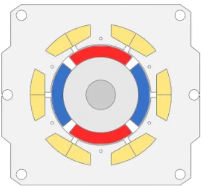
due to different PM magnetization conditions. Fig. 1 shows the motor topology with 6 stator slots and
4 rotor poles.
Impact Analysis of PM magnetization level on
motor performance: simulations and
experimental results
Tiago Staudt, Thiago Akinaga,EMBRACO R&D Department, [email protected], [email protected]
Leonardo Ulian Lopes,
UFSC - Engineering Department, Campus Blumenau, [email protected]
Fernando Maccari, Paulo A. P. Wendhausen
Fig. 1 - Cross-sectional view of the BLDC 6 slots 4 poles motor topology used in the case study.
Details about the electromagnetic design of such motor can be found in [5]. The first part of the
paper presents the methodology used to measure the PM polarization before their assemblies to the
rotor. Then, experimental tests are reported, comparing performance characteristics among different
rotors. Finally, a discussion on raw materials utilization is presented based on a simulation approach.
II. METHODOLOGY
A. Assessing the magnetization conditions: the use of Helmholtz coil for measuring the magnetization level of PM samples
The arc segments used in the BLDC have been magnetized and their polarizations have been
individually measured by means of a Helmholtz coil. Fig. 2 shows the Helmholtz coil used for the
measurements [6].
Fig. 2 - Helmholtz coil from Brockhauss Messtechnik used in the tests.
The magnetic material characterization using the Helmholtz coil evaluates the magnetic properties
of permanent magnets in open-circuit conditions, without applying external magnetic fields to the
samples, hence not influencing their magnetization state. The following properties are measured using
this device at room temperature: Magnetic Flux (V.s).
Magnetic Polarization at the working point (open-circuit) (T).
For the measurements on this device, the following considerations must be taken into account: The PM samples must be in the magnetized state.
They must be lower than 50,0 mm in any direction (for the considered coil).
The magnetization axis must be known.
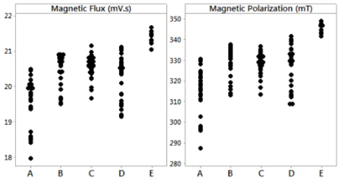
Several groups of ferrite arc segments have been magnetized using different devices and conditions
(A, B, C, D and E). Fig. 3 shows the dispersion of the results for the magnetic flux and polarization
for each group. Differences in the mean value and standard deviation among the groups can be
noticed and, from these results, best and the worst magnetized samples (in terms of magnetic flux)
have been selected to be used in the tests presented in the sequence.
Fig. 3 - Magnetic flux and polarization measured using the Helmholtz coil for ferrite arc segments.
B. Methodology applied to evaluate the impact of PM magnetization tolerances on motor performance
The approach used to analyze the impact of PM magnetization in motor performance seeks to
isolate their effect from other manufacturing tolerances. Therefore, the same stator has been used for
all tests.
Regarding the rotor, four arc segments of alternate polarities (NSNS) are required for each
assembly. The rotor has been prepared with the core produced with silicon-iron steel. The rotor stacks
have been prepared from the same batch and in the same day. The selected PM’s from Fig. 3 have
being separated in two groups: the ones with highest values of polarization and the ones with the
lowest levels. Then, this controlled PM arc segments have been assembled to the rotor stacks to
evaluate the effect of different magnetization levels in motor performance. Fig. 4 shows the three
rotor samples that have been prepared.
Fig. 4 - Picture of the rotor samples under analysis.
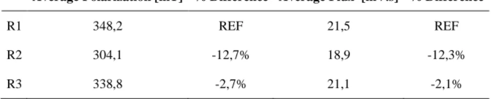
Table I summarizes the average magnetization levels of the PM arc segments in terms of
polarization and flux that have been chosen to assemble each rotor. The average polarization of R1 is
348.2 mT and this value is assumed to be the reference. The average is calculated by considering the
average polarization that is 12.7% below the reference. Sample R3 is 2.7% below the reference. This
nomenclature is used throughout this paper to designate the different rotors under analysis.
TABLE I-AVERAGE MAGNETIZATION FOR THE THREE ROTOR SAMPLES CONSIDERED IN THIS REPORT.
Average Polarization [mT] % Difference Average Flux [mV.s] % Difference
R1 348,2 REF 21,5 REF
R2 304,1 -12,7% 18,9 -12,3%
R3 338,8 -2,7% 21,1 -2,1%
It is important to mention that the polarization levels indicated in Table 1 are measured in
open-circuit using the Helmholtz coil and do not represent directly the PM’s remanence, which is the
polarization in the absence of self-demagnetizing fields. For the simulation considered latter in this
paper, the actual values of Br have been estimated by using the software SPEED [7] by adjusting the
Br coefficient to match the measured and simulated back-emf waveforms
III. EXPERIMENTAL TESTS FOR THE IMPACT ANALYSIS OF PM MAGNETIZATION STATE ON MOTOR’S PERFORMANCE
The following tests have been performed considering a winding temperature of 30 °C +- 5°C: Back-EMF.
Torque versus Current. Efficiency versus Torque. Maximum torque versus speed.
The experimental results are also used to calibrate the simulation model developed in the software
SPEED version 10.02. Once calibrated, the SPEED model is used to estimate the impact of PM
magnetization conditions in raw material utilization for obtaining about the same performance.
A. Back-EMF
1) Back-EMF at 2000 rpm
The measured back-EMF curves at 2000 rpm for the three rotors are shown in Fig. 5.
Fig. 5 - Measured back-EMF for the 3 rotor samples at 2000 rpm.
To better evaluate the results, Fig. 6 shows a zoom in the region of interest for the 3 distinct rotors -150
-100 -50 0 50 100 150
0 10 20 30 40 50 60
Ba
c
k
-EM
F
[V
]
Number of points
at 2000 rpm.
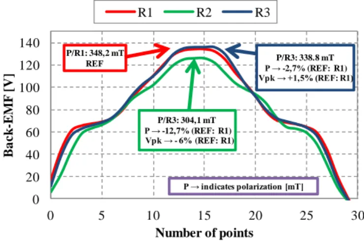
It can be remarked that the samples R1 and R3 have similar waveforms. This is expected, since
their polarizations (P) are similar (2.7 % difference). The R2 sample has roughly 12.7% less flux than
the R1 sample, which represent a peak value in the back-EMF waveform that is 6 % lower.
Fig. 6 - Measured Back-EMF (zoomed) for the 3 rotor versions at 2000 rpm.
2) Measured Back-EMF at 3000 rpm
Similar behavior as identified in Fig. 6 can be verified in Fig. 7 for a zoomed region at 3000 rpm for
the three samples. While the magnetization level is 12.7% lower in R2 sample, the peak difference is
6.5% lower in this sample than it is in the R1.
Fig. 7 - Measured Back-EMF (zoomed) for the 3 rotor versions at 3000 rpm.
B. Torque versus Current at 2000 rpm
The torque is proportional to current and is given by [1]:
(1)
where is the torque constant.
By plotting a torque versus current one can roughly determine the constant for different
machines. In this case, since the stator is the same in all the tests, the PM magnetization level is the
only variable that changes in each rotor. Fig. 8 shows the results from 0.2 up to 0.6 A, which
approximately represents a variation from 1 up to 4 kgf.cm in the electromagnetic torque. 0 20 40 60 80 100 120 140
0 5 10 15 20 25 30
Ba c k -EM F [ V ]
Number of points
R1 R2 R3
P/R3: 338.8 mT
P → -2,7% (REF: R1)
Vpk → +1,5% (REF: R1)
P/R1: 348,2 mT REF
P/R3: 304,1 mT
P → -12,7% (REF: R1)
Vpk → - 6% (REF: R1)
P → indicates polarization [mT]
0 30 60 90 120 150 180 210
0 5 10 15 20
Ba c k -EM F [V ]
Number of points
R1 R2 R3
P/R3: 338.8 mT
P → -2,7% (REF: R1)
Vpk → +1,5% (REF: R1)
P/R1: 348,2 mT REF
P/R3: 304,1 mT
P → -12,7% (REF: R1)
Vpk → - 6% (REF: R1)
To estimate the coefficient for all different rotors, a linear trend line is calculated and the results
are shown in Fig. 8. The R1 sample gives an angular coefficient of , similar to the one
of R3 sample as expected, which gives . Regarding the R2” sample, the
. The factor
indicates that the R2 motor can provides roughly 7,2% less
torque than the R1 one.
Fig. 8 - Torque versus current plot at 2000 rpm: trend lines to obtain coefficient .
C. Efficiency versus Torque curves
Efficiency is one of the most fundamental parameter in motor design. This section investigates the
influence of PM magnetization in this aspect in terms of the produced electromagnetic torque through
experimental tests. To have a clearer overview over the entire torque range, the efficiency is plotted in
terms of the torque for 2000 rpm, 1600 rpm and 3000 rpm for the 3 rotor assemblies.
1) Efficiency versus Torque at 2000 rpm
The first comparison is shown at 2000 rpm in Fig. 9. It is possible to infer that for lower excitation
(around 1 kgf.cm), the iron losses dominate the efficiency curve and the R2 rotor is more efficient
since it has a lower Br. At 2 kgf.cm, the efficiency curve reaches its peak with similar efficiency for
all rotors. At this point, the iron losses and copper losses are nearly equivalent. From this point on, the
copper losses dominates the response, since more current is supplied to the motor to sustain the
required torque. Consequently, the losses are higher for the R2 rotor because of the lower induced
back-emf (for the same torque, more current – and winding losses – are required for the R2 rotor). In the worst analyzed case (4.5 kgf.cm), the efficiency is about 1.5 % lower for the R2 than it is for the
R1 rotor.
R1 = 6.5709x + 0.199 R² = 0.9962
R2 = 6.0972x + 0.134 R² = 0.9961 R3 = 6.5339x + 0.1443
R² = 0.9966
1 1.5 2 2.5 3 3.5 4
0.2 0.3 0.4 0.5 0.6
T
o
rq
u
e
[k
g
f.
c
m
]
Current [A]
Fig. 9 - Efficiency versus torque curve at 2000 rpm.
Efficiency versus Torque at 1600 rpm and 3000 rpm (measured only)
Similar behavior as notice for the 2000 rpm for the efficiency curve can be remarked at 1600 and
3000 rpm as shown in Fig. 10 (1600 rpm) and Fig. 11 (3000 rpm).
Fig. 10 - Efficiency versus torque curve at 1600 rpm.
Fig. 11 - Efficiency versus torque curve at 3000 rpm.
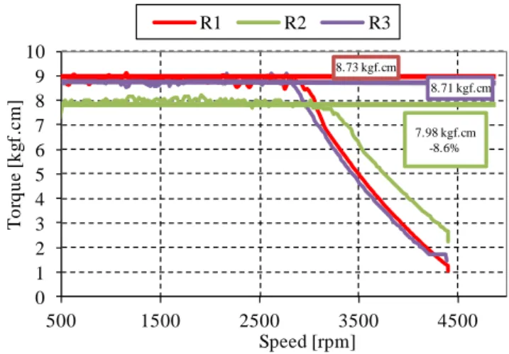
D. Maximum torque output versus speed
The maximum torque versus speed curve is plotted by feeding the motor through the inverter with
rated current while the speed is varied from 4500 rpm up to 0 rpm. Fig. 12 shows the measured 80 81 82 83 84 85 86 87 88 89 90
0.5 0.8 1.1 1.4 1.7 2 2.3 2.6 2.9 3.2 3.5 3.8 4.1 4.4
E ff ic ie n c y [% ] Torque [kgf.cm]
R1 R2 R3
Difference of ~ 1.5 %
80 81 82 83 84 85 86 87 88 89 90
0.5 0.8 1.1 1.4 1.7 2 2.3 2.6 2.9 3.2 3.5 3.8 4.1 4.4
E ff ic ie n c y [% ] Torque [kgf.cm]
R1 R2 R3
80 82 84 86 88 90 92
0.5 0.8 1.1 1.4 1.7 2 2.3 2.6 2.9 3.2 3.5 3.8 4.1 4.4
E ff c ie n c y [ % ] Torque [kgf.cm]
results.
Fig. 12 - Measured maximum torque versus speed curve.
It is possible to remark that the R2 rotor provides 8.6 % less torque than the R1 and R3 rotors. This
result confirms the one inferred from the torque coefficient analysis ( ), which indicated 7.2% less
torque in the R2 motor.
IV. DISCUSSION ON THE IMPACT OVER PERFORMANCE AND RAW MATERIAL UTILIZATION
In order to assess the impact of PM magnetization in raw material utilization, this section presents a
case study as follows. Assuming that the R2 rotor satisfies the application requirements in terms of
torque and efficiency, the stator of R1 rotor is modified so that it has in the final design the same
outcomes of R2 motor. In other words, the extra raw material of R1 rotor is eliminated so that we can
take benefit of a fully saturated PM as the one in rotor R1. This investigation is made by using a
calibrated SPEED model considering the experimental machine presented in this paper.
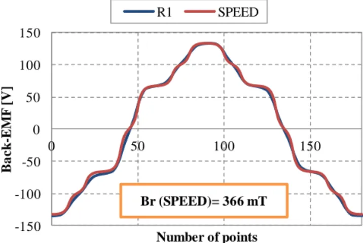
A. Calibration of SPEED software
In order to calibrate the SPEED software for the comparisons that follows, the experimental results
are confronted to the ones obtained from simulation in SPEED. The PM remanence is adjusted in
SPEED in order to obtain a back-EMF waveform that matches the peak of the measured one. Fig. 13
shows a comparison of the R1 sample and the results obtained in SPEED using the Br value of 366
mT. It can be seen that this Br results in a waveform that matches the experimental one with high
accuracy.
0 1 2 3 4 5 6 7 8 9 10
500 1500 2500 3500 4500
T
o
rq
u
e
[k
g
f.
c
m
]
Speed [rpm]
R1 R2 R3
Fig. 13 - Comparison among experimental and simulation results for the BACK-EMF at 2000 rpm and sample R1.
Similarly, the same approach is used for matching the R2 and R3 waveforms with the simulation
from SPEED. Fig. 14 depicts the waveform comparison for R2 sample. A Br = 346 mT provides a
good agreement among the curves.
Fig. 14 - Comparison among experimental and simulation results for the BACK-EMF at 2000 rpm and sample R2.
B. Torque versus speed curve: adjusting the number of turns
Fig. 15 shows the original simulated curves of R1 and R2 rotors performance in terms of torque and
speed. It indicates that it is possible to reduce the R1 torque in about 5.5% in order to get similar
results. Fig. 15 also shows a first attempt to reduce raw material utilization by reducing the number of
turns by 13%. The “NEW R1 temp” motor now has the same torque output as R2 with less turns. -150
-100 -50 0 50 100 150
0 50 100 150
Ba
c
k
-EM
F
[V
]
Number of points
R1 SPEED
Br (SPEED)= 366 mT
-150 -100 -50 0 50 100 150
0 50 100 150
Ba
c
k
-EM
F
[V
]
Number of points
R2 SPEED
Fig. 15 - Original differences for R1 and R2 rotors and the new R1 motor with reduced number of turns.
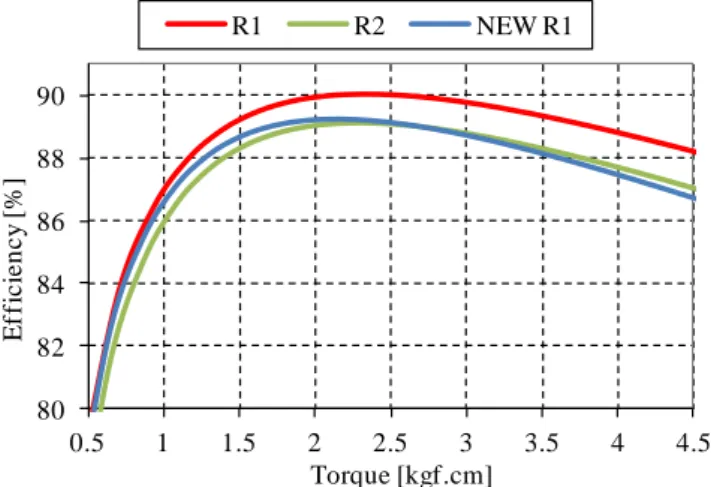
C. Efficiency versus torque curve: reducing the wire diameter to match efficiency
The original efficiency curves for R1 and R2 rotors are compared to the efficiency of the “NEW R1
temp” motor without any other change besides the number of turns. The results are shown in Fig. 16.
Fig. 16 - Original efficiency versus torque curve at 2000 rpm compared to the new motor.
It is noticed that that the efficiency of the “NEW R1 temp” motor is closer to the R2, but we still
have a margin to work with. Therefore, the wire diameter is reduced by 6.6% in order to gain in
copper weight aiming to match R2 efficiency (NEW R1). Fig. 17 depicts the results. It is possible to
remark that these design modifications allow redesigning the R1 motor so that it nearly matches the
performance of the R2 motor in terms of torque production and efficiency. 2
3 4 5 6 7 8 9 10
500 1000 1500 2000 2500 3000 3500 4000 4500
T
o
rq
u
e
[k
g
f.
c
m
]
Speed [rpm]
R2 SPEED R1 SPEED NEW R1 temp SPEED
~ 5.5%
80 82 84 86 88 90
0.5 1 1.5 2 2.5 3 3.5 4 4.5
E
ff
ic
ie
n
c
y
[
%
]
Torque [kgf.cm]
Fig. 17 - Effect of reducing the number of turns and wire diameter for the final design NEW R1.
Table II summarizes the impact on raw materials. There is a decrease of nearly 21 % in cooper
weight by reducing the number of turns and the wire diameter considering narrower tolerances in the
PM arc segments magnetization conditions.
TABLE II–IMPACT ON RAW MATERIAL UTILIZATION.
Copper weight [kg]
R1 / R2 0.3109
NEW R1 0.2457
Diff % -20.97%
V. CONCLUSIONS
This paper addresses the impact of manufacturing tolerances in the magnetization level of ferrite arc
segments on BLDC motor design. The effect is analyzed from a performance point of view and the
best utilization of raw material is discussed using both experimental and simulation results. It has
been found that, for the considered case study, if one can reduce the tolerance margins for
magnetization of ferrite arc segments in the manufacturing line, a significant amount of raw material
can be reduced from the final motor design for the same application requirements. In the considered
case study, an improvement of 12 % resulted in a copper reduction of 21%.
REFERENCES
[1] K. W. Lee, J. Hong, S. B. Lee and S. Lee, "Quality Assurance Testing for Magnetization Quality Assessment of BLDC
Motors Used in Compressors," in IEEE Transactions on Industry Applications, vol. 46, no. 6, pp. 2452-2458, Nov.-Dec. 2010.
[2] M. F. Hsieh, D. G. Dorrell, C. K. Lin, P. T. Chen and P. Y. P. Wung, "Modeling and Effects of In Situ Magnetization of
Isotropic Ferrite Magnet Motors," in IEEE Transactions on Industry Applications, vol. 50, no. 1, pp. 364-374, Jan.-Feb. 2014.
[3] M. Hsieh and S. Yu, "In-situ magnetization of permanent magnet machines considering magnetizer capacity and
connection types," 2015 IEEE Magnetics Conference (INTERMAG), Beijing, 2015, pp. 1-1.
[4] M. F. Hsieh, Y. C. Hsu and P. T. Chen, "Analysis and Experimental Study of Permanent Magnet Machines With
In-Situ Magnetization," in IEEE Transactions on Magnetics, vol. 49, no. 5, pp. 2351-2354, May 2013.
[5] Hendershot, JR., Miller, TJE; Desing of Brushless Permanent-Magnet Machines. ISBN 978-0-9840687-0-8. 2010.
[6] Brockhaus Messtechnik Website. Accessed on 20/04/2015:
http://brockhaus.com/de/messtechnik/messtechnik-fuer-hartmagnetische-werkstoffe/spulen/helmholtzspule/
[7] Miller, TJE, MI McGilp. SPEED PC-BDC 10.02. SPEED laboratory, Glasgow. Computational Dynamic Ltd., 2015.
80 82 84 86 88 90
0.5 1 1.5 2 2.5 3 3.5 4 4.5
E
ff
ic
ie
n
c
y
[%
]
Torque [kgf.cm]