Abstract— An accurate modeling of materials is essential to obtain
reliable results in fields calculation. The Jiles-Atherton approach is widely used for modeling the magnetic hysteresis and depends on its set of five parameters to properly represent material. In this article is proposed an original methodology for obtaining this set of parameters avoiding the derivatives rough calculation and using the calculation of integrals. From the model equations, a new methodology with two nonlinear algebraic systems of five equations in five unknowns is obtained. The initial magnetization curve, the anhysteretic curve and filtering data are not necessary. The proposed methodology also does not restrict the search space of parameters. The parameters assume values in the interval (0,∞). Calculated data were compared with experimental data to validate the methodology. The simulations showed that the proposed method can obtain an accurate set of parameters from a single experimental hysteresis loop and with low computational effort.
Index Terms— Cauchy problem, Maclaurin's series, Magnetic hysteresis, magnetic materials.
I. INTRODUCTION
Several models for scalar modeling of magnetic hysteresis are found in the literature but the
Jiles-Atherton approach has been widely used [1]-[9]. To completely characterize a given material the
Jiles-Atherton model requires the determination of five parameters: ms(A/m), α, a (A/m), k, and c
[10]-[12]. The calculation of these parameters has been performed through different methods
stochastic and deterministic.
Recent research developed by the authors of this article resulted in three different methodologies to
calculate the parameters of the Jiles-Atherton model, based on the knowledge of only one
experimental B-H curve of the material. The three methodologies have the same origin (the equations of Jiles-Atherton); they use the same method (non-linear least squares) to solve an equations system
of infinitely many solutions where the solution is the set of parameters to be calculated; and they were
applied to characterize the same material. The differences between the methodologies will be
highlighted. In the first method, after algebraic manipulation of the Jiles-Atherton equations one
obtains Mirr = Mirr (He (H, B)), and reaches to a nonlinear ordinary differential equation dB / dH = f1
(H, B). The derivative is calculated roughly. The system of equations is written with this last equation.
An Improved Method for Acquisition of the
Parameters of Jiles-Atherton Hysteresis Scalar
Model Using Integral Calculus
Filomena Barbosa R. Mendes1, Jean V. Leite2, Nelson J. Batistela2, Nelson Sadowski2, 1
UTFPR, DAELE, DAMAT, PROFMAT, Pato Branco PR, 85503-390, Brazil, [email protected]
Fredy M. S. Suárez1 2
The derivative of a function B (H) at the point H1 is defined by the
limit,
1
1
10
lim /
H
B H B H H B H H
, when this limit exists. Thus, to improve the
first method, in the case of noisy loops, it is necessary to avoid the derivative calculation. In the
second method (which avoids the derivative calculus) proposed in this paper, after algebraic
manipulation of the Jiles-Atherton equations, one obtains Man = Man (He) and dMan / dHe = f2 (He)
allowing write a linear ordinary differential equation ODE. The Cauchy problem associated with ODE
is solved and its initial value is an experimental magnetic field and magnetic induction. This allows
writing a nonlinear algebraic equation B/μ0-H = f3 (H, B). The integral involved in this algebraic
equation is solved roughly using Maclaurin series. To improve the accuracy are considered the first
ten terms of the series. The equations system is written with this algebraic equation. In order to
improve the second methodology is necessary to avoid rough calculation of integrals. Therefore, the
third methodology was developed. In the third method, after algebraic manipulation of Jiles-Atherton
equations, are obtained directly (without using rough calculations of derivative and integrals) B = B
(He, H). A nonlinear algebraic equation f4 (H, B) is written and used to construct the system of
equations.
For the same material, the different methodologies do not provide, as a result, equal sets of
parameters. It is true that the proposed methodologies have the same origin, but the methodologies
identify the set of parameters by solving different equations systems. The first methodology calculates
parameters based on derivatives rough calculation; the second method calculates parameters based on
power series approximation to solve the integral; the third method is simpler and does not use
derivative or integral to identify the parameters.
Each of the equations systems analyzed in the three methodologies has infinitely many solutions.
Although there are infinitely many solutions, only some of them can be calculated because the main
equations in each methodologies have a division operator (which is inherited from Jiles-Atherton
equations) and hence indeterminate forms can happen avoiding the calculation of all existing
solutions.
In addition, there are five parameters, which can also be seen as five degrees of freedom.
Depending on the value assumed by one of the parameters, the other can be set according to assumed
already value.
The Jiles-Atherton equations originate three methodologies, this is fact, and cannot be seen as a
drawback because the three methodologies give opportunity to calculate several sets of parameters
which are then analyzed based on criteria that facilitate the selection of the set that best represents the
experimental behavior of the material.
In this article, a new and original method to determine the five parameters of Jiles-Atherton
hysteresis scalar model is proposed. Reference [13] proposes an original method to determine the five
B was written in function of magnetic field H and in terms of the derivative of B with respect to the magnetic field. If there are numerical noises added to the measured experimental data then the
calculation of the derivative may be difficult. Despite this, the approach has been used to characterize
different materials and the results show good agreement of measured data and calculated data.
The main contribution of this paper is to improve the method for obtaining the parameters of
Jiles-Atherton model using an inverse model, where the magnetic induction is the independent variable,
and, unlike the previous work, avoiding the use of derivatives calculus in the characterization method.
In summary, the proposed approach can be described as follows. First, the model Jiles-Atherton is
written as a linear ordinary differential equation. Then, the Cauchy problem associated with this
differential form is considered [14]. The initial value of the Cauchy problem is an arbitrary data point
(H0, B0). Then the Cauchy problem is solved using the method of integrating factor [15] and
integration by parts. Finally, the definite integral obtained is solved numerically by Maclaurin series
[16]. The proposed method is simple because the integrand can be represented by polynomial
functions facilitating their integration.
II. MATHEMATICALMODELING
To determine the model parameters a single main equation is obtained (as one can see in appendix)
based on the five equations of Jiles-Atherton and on a constitutive relation [12]. This equation is given
by (1).
The equation (1) is a function of B, H, in that also appear the five parameters of the Jiles-Atherton model. The equation implicitly relating magnetic field and magnetic induction. Knowing the
coordinates of points, magnetic field and magnetic induction, using equation is possible to identify the
five parameters of the model. Another advantage of (1) is the derivative absence.
0 0 0 0
0
/ 1 / 1 /
0 0 0 0
1
/ 1 /
0 0
1
0 0 0 0
0 0 0 0
/ /
1 / / 1 / 1
/ 1 cot / 1 /
/ / 1 cot / 1 /
B H B H k
n
B H k
s n
n n
s
s
B H B H e
c m k e c n B H
B H cm h B H a
a B H cm h B H
0/ 0 1 0 / 0 1 / 0 0 0
/ / 1 B H B H k
a
a B H e
(1)
Where: ms (A/m), α, a (A/m), k, and c are the five material parameters; δ takes the value 1 for the
ascending branch of the hysteresis loop, and the value -1 for the descending branch of the hysteresis
loop; H is the magnetic field; B is the magnetic induction; and µ0 is the magnetic permeability of
vacuum.
III. SOLVINGSYSTEMOFEQUATIONS
Equation (1) can be used to obtain the five parameters of Jiles-Atherton model when an
this operation. Then, 0 = f (H, B) was used to write two systems of non-linear algebraic equations, as can be seen in Fig. 1. The first system represents the ascending branch of the hysteresis loop (Asc.)
when δ = +1. The second system represents the descending branch of the hysteresis loop (Desc.) when
δ = -1. Then points (H0, B0) belonging to the experimental curve are selected. Each system has five
equations in five unknowns. The unknowns are the five parameters of the Jiles-Atherton model.
Finally, each system of equations is solved using the nonlinear least squares method. The parameter
set that represents the material, which corresponds to the experimental hysteresis loop, is the solution
of the equation system.
Fig. 1. System of equations for each branch of the experimental hysteresis loop.
Consider a system of five nonlinear equations given by Fi (x) = f (Hi, Bi) where x = [msαakc] are
the five unknowns, i = 1, ..., 5. The aim is to find a vector x such that Fi (x) = 0. To solve this system
of equations is necessary minimizing the sum of squares. If the sum of the squares is null then the
system of equations is solved. To solve the system was used the Trust-Region-Dogleg algorithm
(TRD) or Trust-Region-Reflective algorithm (TRR) [17], [18] belonging to the nonlinear least squares
method.
The system has infinitely many solutions and is solved by the following method: first, is assigned
an arbitrary initial value for the set of parameters x0 = [ms0 α0a0k0c0]. To the descending branch of
the hysteresis loop select a point with coordinate (H0, B0) belonging to the experimental curve. Five
points with coordinates (H, B) positioned in this branch as can be seen in Fig. 1 are selected. The five points are not positioned considering the most relevant slopes of the branch because (1) does not have
the term dB/dH. The proposed equation f (H, B) evaluated in each selected point (H, B) is writen (this allows to obtain a five-equation system). By solving this system of equations (using the TRD
algorithm or TRR algorithm), a candidate to solution (cs) is obtained.
The candidate to solution above now is used as initial value for the current set of parameters, x0 =
cs. Repeat the procedure for the ascending branch of the experimental hysteresis loop. The point of
coordinates (H0, B0) and the five points of coordinates (H, B) belong to the ascending branch. This
solution is obtained and used as a set of initial parameters for the system.
This procedure is repeated until a certain error criterion is obeyed by candidate to solution, or until
the maximum number of iterations is reached. When a solution is found the simulated hysteresis loop
is calculated and the curve obtained is compared with the measured data. For the set of parameters
representing the material, corresponding to the experimental hysteresis loop, are calculated: mean
squared error (MSE); total accumulated distance calculated considering measured points and
calculated points; and percentage error calculated considering the measured magnetic loss and
calculated magnetic loss.
If the algorithm does not converge, then the initial set of parameters should be changed as well as
the points with coordinates (H0, B0), the error criterion and the maximum number of iterations.
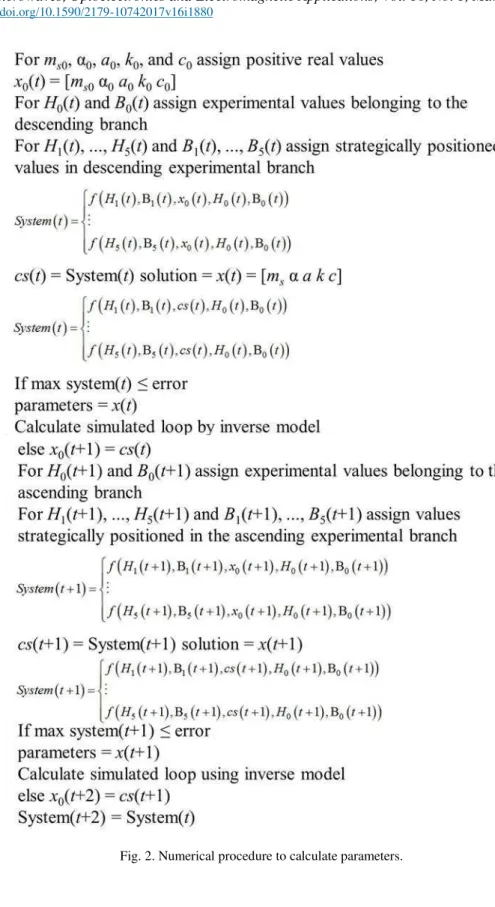
The main steps of the numerical procedure to calculate the parameters of the Jiles-Atherton
hysteresis scalar model are shown in Fig. 2.
IV. APPLICATIONRESULTSOFPROPOSEDMETHODOLOGY
In this section, calculated hysteresis loops are compared to measured hysteresis loops to validate the
proposed methodology. The results were obtained using the proposed methodology and the equations
were solved using the TRD algorithm or TRR algorithm. The experimental data were obtained using
an Epstein frame with closed loop control [19], sinusoidal magnetic induction with frequency of 1 Hz.
Three materials of grain oriented silicon steel cut in the rolling direction were considered, as shown in
Fig. 3-5. A material of grain non-oriented silicon steel cut in the transverse direction was
characterized as can be seen in Fig. 6. A material of non-oriented steel silicon cut in the direction of
45 degrees was analyzed as can be seen in Fig. 7. The corresponding values of the model parameters
(solution) are shown in table I. In the same table the simulation time (t) for obtaining the parameters with a PC i5, 2.67 GHz is given as well as the number of iterations (NI) for each output, the initial set
of parameters used (initial), and initial value used for the Cauchy problem (H0, B0). The parameters
are rapidly obtained and the proposed methodology can be used for fast characterization of materials.
Fig. 3. Calculated results and measured results for material 1: soft loop (TRD).
Fig. 4. Calculated results and measured results for material 2: first case (TRD).
-800 -600 -400 -200 0 200 400 600 800 -1.5
-1 -0.5 0 0.5 1 1.5
Magnetic Field Strength (A/m)
M
a
g
n
e
ti
c
Fl
u
x
D
e
n
s
it
y
(
T)
Simulated Measured
Fig. 6. Calculated results and measured results for material 4: fourth case (TRD).
-500 -400 -300 -200 -100 0 100 200 300 400 500 -1.5
-1 -0.5 0 0.5 1 1.5
Magnetic Field Strength (A/m)
M
a
g
n
e
ti
c
Fl
u
x
D
e
n
s
it
y
(
T)
Simulated Measured
Fig. 7. Calculated results and measured results for material 5: fifth case (TRR).
TABLE I. RESULTS
Case Description Parameters of Material
ms α a k c
Soft
Initial 1.72x10⁶ 1.7x10⁻⁴ 129.8 195 0.47
Solution 1.67x10⁶ 2.38x10⁻⁴ 129.5 89.13 0.51
t (s) 4.31 NI 3
H0,B0 Desc. 19, 1 Asc. -19, -1.1
1o
Initial 1.5x10⁶ 4x10⁻⁴ 200 200 3.12
Solution 1.78x10⁶ 1.54x10⁻⁴ 101.5 81.22 0.34
t (s) 2.56 NI 3
H0,B0 Desc. -15, 0.8 Asc. 14, -0.8
3o
Initial 1x10⁶ 5.0x10⁻⁴ 500 300 0
Solution 1.47x10⁶ 1.36x10⁻⁴ 69.69 48.06 0.16
t (s) 1.97 NI 4
Case Description Parameters of Material
ms α a k c
4o
Initial 1.55x10⁶ 200x10-4 519 460 0.3
Solution 1.55x10⁶ 1.07x10⁻³ 518.4 459.9 0.3
t (s) 2.53 NI 3
H0,B0 Desc. -6, 1.03 Asc. 6, -1.01
5o
Initial 1.3x10⁷ 18x10-4 154 195 0.08
Solution 1.33x10⁶ 7.88x10⁻⁴ 363.71 330.27 0.45
t (s) 2.58 NI 4
H0,B0 Desc. 71, 0.8 Asc. -71, -0.8
TABLE II. SOLUTION QUALITY INDICATORS
Case Solution Quality Indicators
Total Dist. Minimum Dist. Maximum Dist. MSE Error% Soft 4155 1.89x10⁻³ 31.23 10.43 7.11
1o 1111.7 5x10⁻³ 17.86 7.68 3.86
3o 6342.5 3.13x10⁻³ 22.29 4.59 1.53
4o 15581.1 1.94x10⁻³ 73.33 19.00 1.95
5o 15521.4 5.13x10⁻³ 60.89 22.80 0.74
The hysteresis sigmoid soft loop simulated agrees with the experimental data as shown in Fig. 3. As
one can see in Fig. 4-7 the simulated loops also show good agreement with the measured hysteresis
loops.
Table II shows indicators of the solution quality: mean square error (MSE); calculated distance
considering measured points and calculated points (Dist.); and percentage error calculated considering
the measured magnetic loss and calculated magnetic loss (Error%).
The two systems of nonlinear equations presented in the proposed methodology can be solved using
the method of nonlinear least squares (used in adjustment nonlinear curves).
From the equations of Jiles-Atherton hysteresis scalar model and a constitutive relationship were
written two systems of nonlinear equations. The aim is to compute the parameters of Jiles-Atherton
model of the curve that best fits the experimental data of magnetic induction and magnetic field for a
given material. These parameters, which fit (by the nonlinear least squares technique) the nonlinear
function (obtained from the proposed methodology) to a set of experimental points of magnetic
induction and magnetic field, can be identified for example by Trust-Region-Dogleg algorithm or
Trust-Region-Refective algorithm [17].
With characteristic of avoid the derivative calculus, this methodology shows great potential for
reliable and fast identification of the parameters of the Jiles-Atherton model. Although the aim of this
work is the parameters identification of the Jiles-Atherton scalar hysteresis model the method
proposed here can also be used to determine the parameters of the Jiles-Atherton vector model. In this
case the methodology can be used for each main direction of magnetization: longitudinal direction
In [20] - [28], one can see methodologies to determine the parameters of Jiles-Atherton hysteresis
scalar model using algebraic manipulation of the model equations and the application of nonlinear
least squares method to solve the system of equations obtained.
V. CONCLUSION
In this article, a modeling of magnetic hysteresis is presented using the Jiles-Atherton model. A
mathematical model and a new methodology, which requires few experimental data from the
hysteresis loop, are used to evaluate the model parameters. The proposed approach improves the way
in which these parameters are determined avoiding the calculus of derivatives. To our knowledge, this
model which implicitly relates the magnetic field and the magnetic induction has never been proposed
in the literature. Despite the complexity involved in the derivation of the algebraic system and in the
integral calculus by unconventional methods, the final results allows fast computational method
providing reliable hysteresis loop when compared with experimental loops.
APPENDIX
The equations that allows identifying the model parameters are the equations of the Jiles-Atherton
scalar hysteresis model and a constitutive relationship. According to [12] are considered the following
equations:
irr rev
M
M
M
(2)
rev an irr
M
c M
M
(3)coth e
an s
e
H a
M m
a H
(4)
irr an irr
e
dM
M
M
dH
k
(5)e
H
H
M
(6)
0
B
H M
(7)A. Cauchy Problem Associate
Keeping in mind that the purpose of this section is to find the five parameters of the Jiles-Atherton
hysteresis scalar model without using the derived calculation, the mathematical modeling begins
combining (3) and (2): M = Mirr+c(Man-Mirr) that is
1
irr anM
c M
cM
(8)Furthermore, considering (6) we have αM = He-H, that is, M = (He-H)/α which combined with (7)
allows to write B = µ0[H+((He-H)/α)]. From this last equation one obtains: 0
0
1
1
eB
H
H
(9)
0
1
e
H
B
H
(10)On the other hand, equation (8) allows calculating the derivative of magnetization with respect to
the effective magnetic field:
1
irr ane e e
dM
dM
dM
c
c
dH
dH
dH
(11)This way, combining (5) and (11) this gives us:
1
1
anan irr
e e
c c dM
dM
M M c
dH k k dH
(12)
By multiplying (8) by 1/(kδ) it is also true that:
1
irr an
c
M
c
M
M
k
k
k
(13)After that, (12) added to (13) allows write:
1
anan an
e e
c dM
dM M c
M c M
dH k k dH k
, or
an an an
an
e e
M
cM
dM
dM
M
c
c
M
dH
k
k
k
dH
k
that isan an
e e
M
dM
dM
M
c
dH
k
k
dH
(14)Taking into account (4), one can see that Man = Man(He) and dMan/dHe = f(He) that is Man and
dMan/dHe both depend of He, as a result it is stated that (14) is a linear ordinary differential equation of
the first order, with dependent variable M and independent variable He.
Consider the Cauchy problem associated with (14). A Cauchy problem is defined by an equation or
systems of first order equations and an initial condition. From (7) B/µ0 = H+M or M = (B/µ0)-H, as a
result the initial condition will be: M(He0) = M0 = (B0/µ0)-H0.
Concerning (10) He0 = (α/µ0)B0-(α-1)H0 and consequently
00 0 0 0 0
0 0
1
e
B
M H M
B
H M H
(15)
The following Cauchy problem is established:
00 0 0 0 0
0 0 1 an an e e e M dM dM M c
dH k k dH
B
M H M B H M H
B. Solving Cauchy Problem
The method of integrating factor will be used in solving the Cauchy problem. The integrating factor
an
ane e e e
e e
M
dM
dM
M
u H
u H
u H
u H c
dH
k
k
dH
and
e
e
e
e e
dM
M
d
u H
u H
u H
M
dH
k
dH
As u(He) ≠ 0 and M(He) ≠ 0 then
e
e
ee e e
dM
M
du
dM
u H
u H
M
u H
dH
k
dH
dH
In the above equation the terms on the right side are compared with those terms on the left side and
one can conclude that:
e eu H du
dH k that is
ee 1u H
u H k
As d(ln[u(He)])/dHe = u'(He)/u(He) then d(ln[u(He)])/dHe = 1/(kδ). Separating the variables in the
equation above and integrating we then get ʃdln(u(He)) = ʃ[1/(kδ)]dHe, as a result ln(u(He)) =
[He/(kδ)]+cte. Especially for cte = 0 this give us ln(u(He)) = He/(kδ) which also means
u(He) = e He/(kδ)
. The integrating factor is eHe/(kδ).
Equation (14) is multiplied by the integrating factor and this gives us:
e e e e
H H H H
an an
k k k k
e e
M dM
dM M
e e e ce
dH k k dH
(16)
As
e e e
H H H
k k k
e e
dM
M
d
e
e
e
M
dH
k
dH
then we can rewrite (16) ase e e
H H H
an an
k k k
e e
M
dM
d
e
M
e
ce
dH
k
dH
.Integrating the above equation that gives us:
e e e
H H H
an an
k k k
e e
e
M
dM
d e
M
e
dH
c e
dH
k
dH
which also means0
0 0
0
1
e e e e
e e
H H H x H x
an
k k k k
an
H H
dM Me M e M e dx c e dx
k dx
(17)In the second term on right side of (17) is applied integration by parts given by ʃUdV = UV-ʃVdU. For U = ex/(kδ) this gives us dU = (1/(kδ))ex/(kδ)dx. For dV = (dMan/dx)dx then ʃdV= ʃ(dMan/dx)dx that
is V = Man. It is also true that:
0 0 0 1 e e e e e e Hx x x
H H
an
k k k
an an
H H H
dM
c e dx c M e e M x dx
dx k
Combining (18) and (17) one obtains:
0 0 0 0 0 1 ee e e e
e e
e
H
H H H x x H x
k k k k k
an an an
H H H
c
Me M e M e dx c M e e M x dx
k k
or
0 0
0
0 0
1
e e e e e
e
H H H x H H
k k k k k
an an e an e
H
c
Me M e e M x dx cM H e cM H e k k
0 0 0 0 01
1
e e e e e
e
H H H x H H
k k k k k
an an e an e
H
Me
M e
c
M
x e
dx cM
H
e
cM
H
e
k
(19)Both members of equation (19) are multiplied by e-He/(kδ), we then get:
0 0 0 0 01
1
e e e e e e
e
H H H H x H H
k k k k
an an e an e
H
M
M e
c
e
M
x e
dx cM
H
cM
H
e
k
.The total magnetization is isolated of the other variables in the equation above, this gives us:
0 0 0 0 01
1
e e e e e e
e
H H H H x H H
k k k k
an an e an e
H
M
M e
c
e
M
x e
dx cM
H
cM
H
e
k
.Considering the above equation and (4) one can write:
0 0 0 0 0 0 1 1 coth coth cothe e e e
e
e e
H H H H x
k k k
s H
H H
e e k
s s
e e
x a
M M e c e m e dx
k a x
H a H a
cm cm e
a H a H
(20)C. Proposal Relation: Magnetic Induction with Magnetic Field
Once solved the associated Cauchy problem it is important to note that: one can return to original
equations of the model to write an equation that relates the magnetic induction with the magnetic
field, where also appear the parameters of the material. Taking this into account, from equality (7) M
0 0 0 0 0 0 0 0 0 1 1 0 0 0 0 1 1 1 0 0 0 0 0 1 coth 1 coth 1 1 cothB H B H
k
B H B H
x
s k k
B H
s
s
B B
H H e
m x a
c e e dx
k a x
B H a cm a B H B H a cm a
0 0 0 0 0 0 0 1 1 1B H B H
k B H e
(21)The definite integral in (21) is solved by Maclaurin series and one can obtain (1).
ACKNOWLEDGMENT
This work has been supported by UTFPR, Fundação Araucária, SETI, CAPES, and CNPq.
REFERENCES
[1] J. V. Leite, N. Sadowski, P. Kuo-Peng, N. J. Batistela, and J. P. A. Bastos, “The inverse Jiles–Atherton model parameters identification,” IEEE Trans. Magn., vol. 39, pp. 1397–1400, May 2003.
[2] J. V. Leite, N. Sadowski, P. Kuo-Peng, N. J. Batistela, J. P. A. Bastos, and A. A. de Espíndola, “Inverse Jiles-Atherton vector hysteresis model,” IEEE Trans. Magn., vol. 40, no. 4, pp. 1769–1775, Jul. 2004.
[3] D. Lederer, H. Igarashit, A. Kost, and T. Honma, “On the parameter identification and application of the Jiles-Atherton hysteresis model for numerical modelling of measured characteristic,” IEEE Trans. Magn., vol. 35, no. 3, pp. 1211-1214, May 1999.
[4] P. R. Wilson, J. N. Ross, and A. D. Brown, “Optimizing the Jiles–Atherton model of hysteresis by a genetic algorithm,” IEEE Trans. Magn., vol. 37, no. 2, pp. 989-993, Mar. 2001.
[5] J. V. Leite, S. L. Avila, N. J. Batistela, W. P. Carpes Jr., N. Sadowski, P. Kuo-Peng, and J. P. A. Bastos, “Real coded genetic algorithm for Jiles–Atherton model parameters identification,” IEEE Trans. Magn., vol. 40, no. 2, pp. 888-891, Mar. 2004.
[6] S. Cao, B. Wang, R. Yan, W. Huang, and Q. Yang, “Optimization of hysteresis parameters for the Jiles-Atherton model using a genetic algorithm,” IEEE Trans. App. Supercond., vol. 14, no. 2, pp. 1157-1160, Jun. 2004.
[7] F. R. Fulginei and A. Salvini, “Softcomputing for the identification of the Jiles–Atherton model parameters,” IEEE Trans. Magn., vol. 41, no. 3, pp. 1100-1108, Mar. 2005.
[8] M. Toman, G. Stumberger, and D. Dolinar, “Parameter identification of the Jiles–Atherton hysteresis model using differential evolution,” IEEE Trans. Magn., vol. 44, no. 6, pp. 1098-1101, Jun. 2008.
[9] A. Corana, M. Marchesi, C. Martini, and S. Ridella, “Minimizing multimodal functions of continuous variables with the ‘simulated annealing’ algorithm,” ACM Transactions on Mathematical Software, vol. 13, pp. 262-280, Sept. 1987. [10]D. C. Jiles and D. L. Atherton, “Theory of ferromagnetic hysteresis,” Journal of Magnetism and Magnetic Materials,
vol. 61, pp. 48-60, 1986.
[11]D. C. Jiles, J. B. Thoelke, and M. K. Devine, “Numerical determination of hysteresis parameters for the modeling of magnetic properties using the theory of ferromagnetic hysteresis,” IEEE Trans. Magn., vol. 28, pp. 27–35, Jan. 1992. [12]N. Sadowski, N. J. Batistela, J. P. A. Bastos, and M. Lajoie- Mazenc, “An inverse Jiles-Atherton model to take into
account hysteresis in time stepping finite element calculations,” IEEE Trans. Magn., vol. 38, no. 2, 2002. [13]F. B. R. Mendes, J. V. Leite, N. J. Batistela, N. Sadowski, and F. M. S. Suárez, “A new methodology to obtain the
[14]J. Manuel Sotomayor Tello, “Lições de equações diferenciais ordinárias,” Rio de Janeiro: Instituto de Matemática Pura e Aplicada, Projeto Euclides, 1979, pp. 5-7.
[15]Jaime E. Muñoz Rivera, “Cálculo diferencial II & equações diferenciais,” Textos de graduação. Petrópolis. Editora Gráfica Rondon Ltda, 2007, pp. 35-36.
[16]Norman B. Haaser, Joseph P. Lasalle, and Joseph A. Sullivan, “Análisis matemático 2,” Curso Intermedio, vol. 2. México. Editoral Trillas, 1970, pp. 517.
[17][Online]. Available: http://www.mathworks.com/help/optim/ug/equation-solving-algorithms.html.
[18]Rodrigo M. Rosa, “Estudo e implementação do método dogleg para programação não linear,” Trabalho de conclusão de curso Bacharelado Matemática, UFSC, Florianópolis, SC, 2005.
[19]N. J. Batistela, “Caracterização e modelagem eletromagnética de lâminas de aço ao silício,” Tese Doutor em Engenharia Elétrica, CTC, UFSC, Florianópolis, SC, 2001.
[20]F. B. R. Mendes, J. V. Leite, N. J. Batistela, N. Sadowski, and F. M. S. Suárez, “Uma nova metodologia para obtenção de parâmetros do modelo de histerese de Jiles-Atherton,” in MOMAG 2012 Anais de evento, João Pessoa, 2012. [21]F. B. R. Mendes, J. V. Leite, N. J. Batistela, N. Sadowski, and F. M. S. Suárez, “An improved methodology for
obtaining Jiles-Atherton hysteresis model parameters,” in COMPUMAG 2015 Proceedings, Montréal, 2015.
[22]F. B. R. Mendes, J. V. Leite, N. J. Batistela, N. Sadowski, and F. M. S. Suárez, “Uma nova metodologia para obtenção dos parâmetros do modelo escalar de histerese de Jiles-Atherton,” in MOMAG 2016 Anais de evento, Porto Alegre, 2016.
[23]F. B. R. Mendes, J. V. Leite, N. J. Batistela, N. Sadowski, and F. M. S. Suárez, “Uma metodologia aprimorada para obtenção dos parâmetros do modelo escalar de histerese de Jiles-Atherton,” in MOMAG 2016 Anais de evento, Porto Alegre, 2016.
[24]F. B. R. Mendes, J. V. Leite, N. J. Batistela, N. Sadowski, and F. M. S. Suárez, “Uma metodologia simplificada para a obtenção dos parâmetros do modelo escalar de histerese de Jiles-Atherton,” in MOMAG 2016 Anais de evento, Porto Alegre, 2016.
[25]F. B. R. Mendes, J. V. Leite, N. J. Batistela, N. Sadowski, and F. M. S. Suárez, “Inserção do sexto parâmetro no modelo escalar de histerese de Jiles-Atherton e metodologia para identificação dos parâmetros,” in MOMAG 2016 Anais de evento, Porto Alegre, 2016.
[26]F. B. R. Mendes, J. V. Leite, N. J. Batistela, N. Sadowski, and F. M. S. Suárez, “A new method for parameters obtaining of Jiles-Atherton hysteresis scalar model,” in CEFC 2016 Proceedings, Miami, 2016.
[27]F. B. R. Mendes, J. V. Leite, N. J. Batistela, N. Sadowski, and F. M. S. Suárez, “A simplified method for acquisition of the parameters of Jiles-Atherton hysteresis scalar model without use of derivatives,” in CEFC 2016 Proceedings, Miami, 2016.