Abstract— A design of a blade antenna embedded in low-cost dielectric substrate (FR4) and operating at 4.97 GHz is the subject of this paper. The antenna design is accomplished using parametric
analysis in the HFSSTM software, where the antenna dimensions are
changed and it is observed how the changes affect figures-of-merit like input impedance, reflection coefficient and radiation patterns. The antenna prototype is presented, as well as, a comparison between experimental and theoretical results.
Index Terms—antenna, blade, monopoles, embedded
I. INTRODUCTION
One of the most installed antenna on aircraft is the monopole [1]. Although cylindrical monopoles
are easy to manufacture, they have narrow bandwidth [2], whereas planar monopoles provide more
bandwidth and emerge as option to overcome the cylindrical monopole limitation [3].
The blade antenna is classified as wide bandwidth planar monopole and presents aerodynamic
features for aeronautic application [1]. However, antennas on aircraft are exposed to climate
variations, that creates a need to protect the radiator element with some structure less interfering in the
electromagnetic waves [4]. This structure is known as radome.
In this work, the radiator element is presented embedded in the material FR4, which serves as
radome. Considering that radiator element geometry can be designed in different shapes, the use of a
radome impedes to figure out what is the exact radiator geometry. Hence, it is a designer
responsibility uses predefine topologies as starting point for a blade design. Based on that, the
proposed antenna started with predefined shapes presented in [6,7] and it was modified to get it
operating at 4.97 GHz.
The optimized antenna dimensions were achieved through the parametric assessment on the project
variables, and how those variables influence on the radiation and electrical characteristics of the
antenna. The proposed antenna shall operate on the TCAS (Traffic Collision Avoidance System):
bandwidth 960 MHz – 1220 MHz with input impedance of 50 Ω [5]. With the dimensions optimized a
prototype was manufactured and electromagnetic measurements were conducted on the prototype and
with it installed on metallic cylinder. The cylinder represents an aircraft airframe.
Considering the available resource of the laboratory, a frequency scaling process was adopted to
Design of a Blade Antenna Embedded in
δow
-
Cost Dielectric Substrate
Waleska F. Silva, I. Bianchi and Tiago P. Santos
Laboratory of Antennas and Propagation - LAP, Technological Institute of Aeronautics - ITA, Pr. Mal. Eduardo Gomes, 50 12228-900 São José dos Campos – SP, Brazil, [email protected], [email protected],
represented on the metallic cylinder radius. Therefore, it was possible design a blade antenna
operating at 4.97 GHz (4.38 - 5.56 GHz). Since the aircraft comprises of large structure, the
conventional method FEM (Finite Element Method), available on HFSSTM, becomes inefficient, due
to amount of time, computer processing and memory spent in the simulation. Thus, the antenna
analysis on cylinder was accomplished by a combination of MoM (Method of Moments) and FEM,
known as hybrid method (FEM-MoM) [8 - 10].
In the next sections, it will be presented the antenna geometry, parametric studies and the prototype
with its theoretical and experimental results.
II. ANTENNA GEOMETRY
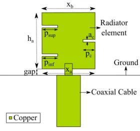
The Fig. 1 shows the first blade antenna proposed. The lengths xa and xb, gap, probe position (p),
slot width (ac), radome presence and ground plan dimensions were changed in order to observe the
effects on the input impedance, reflection coefficient magnitude, impedance bandwidth (-10dB return
loss condition) and radiation pattern. All three slots have the same width (ac).
Fig. 1. Initial blade antenna.
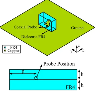
After the parametric assessments on the blade antenna proposed on Fig. 1, it was reached in the
model of Fig. 2, where it’s also presented the radiator element embedded in dielectric substrate and both on a square ground plan. This dielectric is constituted by two FR4 layers ( r = 4.4; tan = 0.02),
with thickness h = 3.2 mm. On one layer it was printed the radiator element, while the other servers as
Fig. 2. Model created on HFSSTM and the superior view of the two FR4 layers attached.
III. PARAMETRIC STUDIES
The HFSSTM was used to optimize the antenna dimensions starting from the geometry presented in
Fig. 1. Initially, the radiator length started in ha = 0.125λ0 [7], however this length was not producing
the best impedance matching at 4.97 GHz. Then, the length was adjusted to 0.156 λ0 to get the best
antenna performance.
The parametric analysis was focused on the search for the best impedance matching considering the
reflection coefficient magnitude.
Next, it is described the influence of the project variables, and the search for optimal antenna
dimensions to construct a prototype compliant with the specifications.
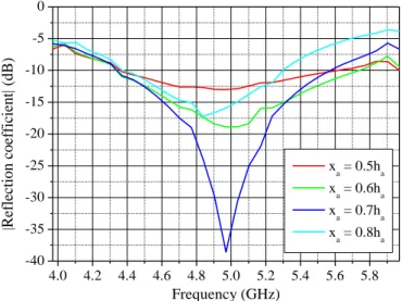
A. Influence of xa and xb on antenna parametric analysis
In this section, the dimensions xa and xb exhibited on Fig. 1 are evaluated. The Figs. 3 and 4 show
how the reflection coefficient magnitude is affected with xa and xb changes. In this analysis, while xa
was changed, xb, ha, psup, pinf, pc, gap and ac were kept unchanged, and while xb was changed, xa, ha,
4.0 4.2 4.4 4.6 4.8 5.0 5.2 5.4 5.6 5.8 -40
-35 -30 -25 -20 -15 -10 -5
xa = 0.5ha xa = 0.6ha
xa = 0.7ha xa = 0.8ha
|
Reflection coefficient|
(dB)
Frequency (GHz)
Fig. 3. Reflection coefficient magnitude with xa variation.
4.0 4.2 4.4 4.6 4.8 5.0 5.2 5.4 5.6 5.8
-40 -35 -30 -25 -20 -15 -10 -5 0
xb = 0.10ha xb = 0.15ha
xb = 0.20ha xb = 0.25ha
|Reflection coefficient| (dB)
Frequency (GHz)
Fig. 4. Reflection coefficient magnitude with xb variation.
A xa variation caused a more pronounced degradation in the reflection coefficient magnitude, as
depicted in Fig. 3, while xb variation resulted in a shifting in frequency, as can be seen in Fig. 4.
Analyzing the operating frequency, the value xa shall be equal to 0.7ha. Considering the new value
for xa the value for xb, which presented best impedance matching, shall be 0.25ha.
B. Gap influence
The Fig. 5 demonstrates how the reflection coefficient magnitude is changed with the gap variation.
It is possible to observe that a gap variation affects the impedance matching, as well as, a frequency
4.0 4.2 4.4 4.6 4.8 5.0 5.2 5.4 5.6 5.8 -40
-35 -30 -25 -20 -15 -10 -5 0
gap = 0.5 mm gap = 1.0 mm gap = 1.5 mm gap = 2.0 mm
|
Reflection coefficient|
(dB)
Frequency (GHz)
Fig. 5. Reflection coefficient magnitude with gap variation.
C. Probe position influence
The Fig. 6 provides a view of how the reflection coefficient magnitude is affected with the probe
position (p) variation.
4.0 4.2 4.4 4.6 4.8 5.0 5.2 5.4 5.6 5.8
-40 -35 -30 -25 -20 -15 -10 -5 0
p = 1 mm
p = 2 mm
p = 3 mm
p = 4 mm
|
Reflection coefficient|
(dB)
Frequency (GHz)
Fig. 6. Reflection coefficient magnitude with probe position variation.
Similar to the gap variation, a probe position change also affects the impedance matching. The
probe position which resulted in the best impedance matching was p = 2mm.
D. Slots width influence
The Fig.7 depicts the change on the reflection coefficient with slots width variation (ac).
Considering the frequency of operation, the slot width which produced the best impedance
4.0 4.2 4.4 4.6 4.8 5.0 5.2 5.4 5.6 5.8 -40
-35 -30 -25 -20 -15 -10 -5
ac = 0.2 mm
ac = 0.3 mm
ac = 0.4 mm
ac = 0.5 mm
ac = 0.6 mm
|Reflection coefficient|
(dB)
Frequency (GHz)
Fig. 7. Reflection coefficient magnitude with slots width variation.
E. Radome influence
In this case, the analysis was performed with and without radome. As presented on the Fig. 8 the
inclusion of the radome decreases the bandwidth, while the radome absence produces more bandwidth
with frequency shifting.
4.0 4.5 5.0 5.5 6.0 6.5 7.0 7.5 8.0
-45 -40 -35 -30 -25 -20 -15 -10 -5 0
6.25 GHz
With radome Without radome
|
Reflection coefficient|
(dB)
Frequency (GHz) 4.97 GHz
Fig. 8. Reflection coefficient magnitude with and without radome.
F. Ground plan influence
The Fig. 9 shows the behavior of reflection coefficient magnitude with variation of ground plan
area (A). It was observed that as bigger as the ground plan area becomes, the coefficient magnitude
increases to below of -30 dB, at operating frequency. The ground plan contribution is insignificant on
4.00 4.25 4.50 4.75 5.00 5.25 5.50 5.75 6.00 -55 -50 -45 -40 -35 -30 -25 -20 -15 -10 -5 0
A = 150 x 150 mm2 A = 250 x 250 mm2 A = 350 x 350 mm2
|Reflection coefficient|
(dB)
Frequency (GHz)
Fig. 9. Reflection coefficient magnitude with ground plan variation.
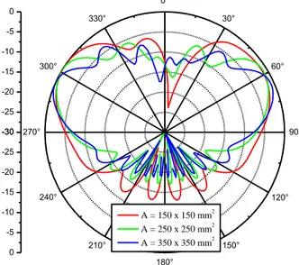
-30 -25 -20 -15 -10 -5 0 0° 30° 60° 90° 120° 150° 180° 210° 240° 270° 300° 330° -30 -25 -20 -15 -10 -5 0
A = 150 x 150 mm2 A = 250 x 250 mm2 A = 350 x 350 mm2
Fig. 10. Radiation pattern in yz plane with ground plan variation.
It was verified considerable changes in the radiation pattern in function of ground plan variation as
can be seen on the plot of yz plane at Fig. 10. It was perceived a reduction of back lobe radiation
patterns as the ground dimensions was increased.
IV. BLADE ANTENNA ON CYLINDER
The analysis of a blade antenna on metallic cylinder representing an airframe of aircraft is the scope
on this section. It is important to emphasize that computational solution takes considerable time and
consumes a lot of RAM memory when it is necessary to simulate antenna on large electrical structure,
like an airframe. Therefore, to reduce simulation time keeping accurate results, the hybrid method
(FEM-MoM) was applied.
To consider the cylinder effects on antenna radiation characteristics using HFSSTM hybrid method,
it was necessary assembly antenna/cylinder as depicted on Fig. 11, where antenna was covered with
an air box type FE-BI boundary, while the metallic cylinder was defined as IE (Integral Equation)
Fig. 11. Blade antenna on metallic cylinder at HFSSTM.
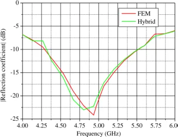
Comparisons between conventional method (FEM) and hybrid method are illustrated through the
graphics of reflection coefficient magnitude, input impedance and radiation patterns in the Fig. 12 and
Fig.13.
4.00 4.25 4.50 4.75 5.00 5.25 5.50 5.75 6.00
-25 -20 -15 -10 -5 0 FEM Hybrid |Re fle c ti on c oe ff ic ie nt| (dB) Frequency (GHz)
Fig. 12. Comparison the results of reflection coefficient magnitude for different numerical methods.
-30 -25 -20 -15 -10 -5 0 0° 30° 60° 90° 120° 150° 180° 210° 240° 270° 300° 330° -30 -25 -20 -15 -10 -5 0 FEM Hybrid -30 -25 -20 -15 -10 -5 0 0° 30° 60° 90° 120° 150° 180° 210° 240° 270° 300° 330° -30 -25 -20 -15 -10 -5 0 FEM Hybrid
(a) (b)
The main antenna figures-of-merit do not differentiate substantially when compared both numerical
methods.
The simulations were performed on Xenon® computer with 192 G RAM and clock 2.4 GHz, with 5
steps of convergence and 38 points, and in the interval of 4 to 8 GHz. The comparison between these
numerical techniques considering simulation time and RAM memory usage is shown on Tab. I.
TABLE I. COMPARISON OF NUMERICAL METHODS FOR THE BLADE ANTENNA ON AIRFRAME.
Resource
Hybrid
FEM
Time
1,176 minutes
2,490 minutes
RAM memory
3.6 G
4.5 G
It was observed a reduction of 20% in RAM utilization while the simulation time became almost
twice faster when used the hybrid method.
V. PROTOTYPE
After finished the parametric studies, the optimal antenna dimensions for a best impedance
matching were those values shown in Tab. II.
TABLE II. VALUES OF THE BLADE ANTENNA
Parameter Value
ha 0.156λ0
xa 0.7ha
xb 0.25ha
pc 1 mm
pinf 10 mm
psup 2 mm
p 2 mm
gap 1 mm
ac 0.4 mm
Using the Prototype System Quick Circuits available at LAP/ITA, the pieces of antenna were
manufactured, as evidenced by the Fig. 14: FR4 layers (one with radiator element and other as
protection) and a supporting plate.
To support the FR4 layers and coaxial probe, it was used a plate of Arlon CuClad ( r = 2.55, tan =
0.0018) with thickness of 0.762 mm. To short-circuit the inferior and superior faces and to avoid wave
guiding were inserted pins, as displayed on the Fig. 14. Although the plate is supporting the layers, it
(a)
(b)
Fig. 14. Prototype without radome (a) and with radome (b).
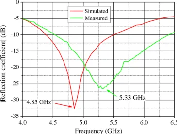
Then, the two FR4 layers were glued to construct the radome, but having precautions for not
deposit material on the radiator element. Measurements on the prototype were carried out to examine
the reflection coefficient magnitude, as well as, comparison with simulated model. These results can
be seen in the Fig. 15.
4.0 4.5 5.0 5.5 6.0 6.5
-35 -30 -25 -20 -15 -10 -5 0
Simulated Measured
|
Reflection coefficient|
(dB)
Frequency (GHz)
4.85 GHz 5.33 GHz
Fig. 15. Comparison of reflection coefficient magnitude for theoretical and prototype models.
The difference raised through the Fig. 15 is associated with variation of electrical permittivity of the
substrate (FR4) according [11, 12], or the presence of air between the dielectric layers. Both
A. Electrical permittivity variation
The Fig. 13 displays the variation of reflection coefficient with electrical permittivity of FR4.
4.0 4.5 5.0 5.5 6.0 6.5
-40 -35 -30 -25 -20 -15 -10 -5 0
4.75 GHz
4.85 GHz
r = 4.0
r = 4.4
r = 4.7
|
Reflection coefficient|
(dB)
Frequency (GHz)
5.05 GHz
Fig. 16. Comparison of reflection coefficient magnitude with variation of FR4 permittivity.
Based on the graphic interpretation it is evidenced a frequency shifting to higher values when FR4
with lower electrical permittivity are used.
B. Space between layers
The method used to join the two FR4 dielectric layers and to solder the probe on the radiator
element resulted in air between the layers. Thus, aiming to analyze what could be the effects of this
gap of air in the input impedance, it was held an experiment with this air gap variation looking its
influence on the reflection coefficient. The results are presented on the Fig. 17, for antenna with the
ground plan illustrated in the Fig. 14.
4.0 4.5 5.0 5.5 6.0 6.5
-55 -50 -45 -40 -35 -30 -25 -20 -15 -10 -5 0
Measured dair = 0 mm
dair = 0.25 mm
dair = 0.30 mm
dair = 0.35 mm
|Reflection coefficient|
(dB)
Frequency (GHz)
Simulated
Fig. 17. Comparison of reflection coefficient magnitude with gap variation between the dielectric layers.
Looking the results on the Fig. 17, it is possible to say that the air gap increase moves the center
frequency to higher values that the value specified on the requirement.
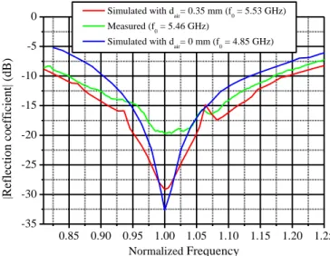
Considering the antenna with ground plan (A = 250 x 250 mm2) and space between the FR4 layers
frequency. Where f0 represents the frequency used to normalize.
0.85 0.90 0.95 1.00 1.05 1.10 1.15 1.20 1.25
-35 -30 -25 -20 -15 -10 -5
0 Simulated with dair= 0.35 mm (f0 = 5.53 GHz)
Measured (f0 = 5.46 GHz)
Simulated with dair= 0 mm (f0 = 4.85 GHz)
|
Reflection coefficient|
(dB)
Normalized Frequency
Fig. 18. Comparison of the reflection coefficient magnitude for experimental and theoretical models when the antenna is on large ground.
It is observed that the prototype presents an impedance bandwidth nearly 1.82 GHz (-10dB return
loss condition), representing 33% in relation to the best impedance matching.
The last comparison is the antenna blade prototype in a ground plane cylindrical, shown in Fig. 19.
This is a hollow metallic cylinder with 250mm of radius. The antenna was fixed on the center of
cylinder.
Fig. 19. Prototype of blade antenna on metallic cylinder.
The results of reflection coefficient magnitude for experimental and theoretical models are
presented in the Fig. 20. In this case, it was considered FR4 relative electric permittivity r = 4.4 and
4.0 4.5 5.0 5.5 6.0 6.5 7.0 -40
-30 -20 -10 0
5.45 GHz
Simulated Measured
|Re
fle
cti
on c
oe
ff
ic
ie
nt| (dB)
Frequency (GHz) 5.30 GHz
4.73 GHz 6.28 GHz
Fig. 20. Comparison of reflection coefficient magnitude for theoretical and prototype models of antenna on metallic cylinder.
The results presented a difference of 150 MHz between the points of best matching. However, in
terms of impedance bandwidth, they are practically the same and the best point of matching is bellow
-20dB, for both cases. Checking the results obtained against the requirements of TCAS, the
impedance bandwidth complies with it is necessary to the service.
Using scaling process, it was achieved a bandwidth of 370MHz, which satisfies the bandwidth
specification for TCAS. However, the lower frequencies of TCAS service are out of the bandwidth
achieved on Fig. 20. Therefore, the antenna optimization is necessary on the cylindrical ground plan
to attend all requirements.
VI. CONCLUSION
In this work, it was demonstrated how the parameters to construct an antenna can influence on the
reflection coefficient magnitude. It is also shown that a ground plan variation produced impacts on the
radiation patterns of the yz plane.
Measurements on prototype revealed divergences in reflection coefficient magnitude when
compared experimental and theoretical models. These divergences are due to variation of FR4 relative
electrical permittivity and/or the space created between the layers in function of solder or glue
accumulation. However, taking these factors to the simulation scenario is possible to see a theoretical
model behaving as the prototype.
Thus, improving the construction techniques for the feeder and measuring the permittivity of FR4,
is possible to build a prototype operating in the design frequency.
The impedance bandwidth achieved for the blade antenna on cylinder was nearly 31.2% while the
impedance bandwidth of TCAS is 23.8%.
It was verified by simulations that hybrid method (FEM-MoM) is the best choice to analyze
structures electrically large, besides that, the simulation time reduced in twice when compares with
the conventional method (FEM) and it was spent 20% less of RAM memory. Considering the
with more complete aircraft with engines and wings, this advantage tends to be much more
pronounced in favor of hybrid technique.
ACKNOWLEDGMENT
The authors would like to thank CNPq for sponsoring project no. 131461/2014-1.
REFERENCES
[1] Macnamara, T. Introduction To Antenna Placement And Installation. Chichester, West Sussex, U.K.: Wiley, 2010.
[2] Balanis, C. A. Antenna Theory: Analysis and Design, 3nd, New York: John Wiley & Sons Ltd., 2005.
[3] Kumar, Girish, and K. P Ray. Broadband Microstrip Antennas. Boston: Artech House, 2003. Print.
[4] Nair, R. U.; Jha, R. M. Electromagnetic Design and Performance Analysis of Airbone Radomes: Trends and
Perspectives [Antenna Applications Corner]. IEEE Antennas and Propagation Magazine. v. 56, p. 276 – 298, Ago 2014.
[5] Sensor system, Inc., Data sheet: L-Band S65-5366- Series, 2004.
[6] SANTOS, Tiago Pereira. Análise de Monopolos Faixa Larga utilizados em Aeronaves. 2015. 98f. Dissertação
(Mestrado em Engenharia Aeronáutica e Mecânica) – Instituto Tecnológico de Aeronáutica, São José dos Campos.
[7] Ono, M.; Takeichi, T. A One-Eighth-Wave Blade Antenna With Metal Leading Edge. 1974. IEEE Antennas and
Propagation Society International Symposium. v. 12, p. 225 – 228, Jun 1974.
[8] Yan, Y. Zhao, LIANG, C. H. Analysis of wire antenna around dielectric or coated object using parallel MoM-PO
technique. IET International Radar Conference 2013. P. 1 – 6, Apr 2013.
[9] LIU, Z. L.; WANG, C. F. An efficient iterative MoM-PO hybrid method for analysis of an onboard wire antenna array
on a large-scale platform above an infinite ground. IEEE Antennas and Propagation Magazine. v. 55, n. 6, p. 69 – 78,
Dez 2013.
[10]BECKER, A., HANSEN, V. Hybrid(3): combining the time-domain method of moments, the time-domain geometrical
theory of diffraction and the FDTD. IEEE Antennas and Propagation Society International Symposium. v. 2A, p. 94 –
97, Jul 2005.
[11]Ammann, M. A. Comparasion of Some Low Cost Laminates for Antennas Operating in the 2,4 GHz ISM Band. IEE
Colloquium on Low Cost Antenna Technology. v. 3, p. 1 – 3, London, 1998.
[12]NASCIMENTO, D. C., Antenas para Comunicações Móveis. 2007.169f. Tese (Mestrado em Engenharia Eletrônica e