Brazilian Microwave and Optoelectronics Society-SBMO received 15 Sep 2016; for review 16 Sep 2016; accepted 28 Dec 2016
Abstract— The single phase equivalent circuit is largely used to model the three-phase induction motors in steady-state operation and under sinusoidal balanced voltages. Depending on the desired application, the circuit may or may not represent core losses, a double cage or even the variation of parameters due to skin effect and saturation. However, the determination of the circuit parameters through standard methods, such as those described in IEEE Standard 112, may not be possible in many situations given the lack of the necessary resources. This paper presents initially a survey on the determination of circuit parameters from alternative methods, i.e., non-standard tests. Special focus is given to methods which employ only data usually provided by manufacturers on catalogs and nameplates. Six analytical methodologies used in the context of efficiency estimation at steady-state operation are assessed, compared and then combined in order to improve results. The assessment is based on the closeness of the resulting parameter values to reference values and on the inexistence of absurd results, such as negative electrical resistances. The combination of methods has improved the accuracy of calculations for the studied motors.
Index Terms—Equivalent circuit, Parameter value estimation, Manufacturer data, Three-phase induction motor.
I. INTRODUCTION
Three-phase induction motors (TIM) operating under steady-state regime are commonly modeled
using a per phase equivalent circuit, which enables the calculation of quantities such as line current,
power factor, input and output power and efficiency simply as a function of supply voltage, frequency
and slip. The circuit parameter values are traditionally determined through tests described on IEEE
Standard 112 [1], such as no load and locked rotor tests. Although such procedures provide reliable
results, their requisites may be impractical in some places or situations. First, the necessary
instrumentation is not often available where the motor is operating, thus demanding the transference
Estimation of Three-Phase Induction Motor
Equivalent Circuit Parameters from
Manufacturer Catalog Data
Carlos A. C. Wengerkievicz, Ricardo de A. Elias, Nelson J. Batistela, Nelson Sadowski, Patrick Kuo-Peng
GRUCAD/EEL/UFSC, P.O. Box 476, 88040-970, Florianópolis, Santa Catarina, Brazil, c.a.correa, [email protected], jhoe.batistela, nelson.sadowski, [email protected]
Sandro C. Lima, Pedro A. da Silva Jr.
GERAC/IFSC, Rua José Lino Kretzer 608, 88103-310, São José, Santa Catarina, Brazil, [email protected], [email protected]
Anderson Y. Beltrame
of the machine to a testing site or laboratory. Second, the necessary interruption in the operation of the
motor is undesired in critical industrial processes. Finally, the knowledge of the circuit parameter
values may be desired prior to acquisition for simulation of even didactic purposes.
These situations have motivated the development of alternative methods for parameter values
determination, ranging from analytical calculations based on nameplate data to frequency response
analysis. The estimated model is destined to various applications, e.g., efficiency assessment and
starting simulation, which also define the details. A particular group of methods, based on information
provided by manufacturers on catalogs or nameplates, stands out in steady-state applications for its
simplicity and its nonintrusive characteristic.
This paper presents a review on parameter values estimation of the equivalent circuit of three phase
induction motors based on data provided by manufacturers on catalogs, with special interest on those
dedicated to efficiency estimation. Section II consists on an overview of methods for parameter
identification in several contexts. Section III summarizes the main methods for equivalent circuit
determination from catalog data by analytical and numerical means. On Section IV, the analytical
methods described on the previous section are applied to a group of motors and their performance is
assessed and compared.
II. OVERVIEW OF ALTERNATIVE METHODS FOR PARAMETER DETERMINATION
A. TIM Models on bibliography
According to [2], methods for identification of TIM parameter values can be classified as:
1. Calculation from construction data: requires the detailed knowledge of the machine’s geometry
and of the properties of the employed materials, besides software for electromagnetic
calculation. It is considered to be the most precise procedure, although costly, and it is
employed basically by manufacturers, designers and researchers.
2. Estimation based on steady-state motor models: the parameter values are obtained through the
solution of equations derived from state-models employing data from tests, measurements or
provided by manufacturers. This class includes the standard testing methods.
3. Frequency-domain parameter estimation: the parameter values are estimated from the transfer
function observed during tests. It is not a common industry practice.
4. Time-domain parameter estimation: the parameter values are adjusted so as the response
calculated with a system of differential equations fits the observed time response.
5. Real-time parameter estimation: commonly applied to controllers for continuous tuning of
parameters of simplified models, compensating parameter variation due to temperature change,
saturation and other effects in the machine.
This work focuses on methods belonging to the second group, especially on those employing data
provided by manufacturers on nameplates or technical catalogs. These data contain information of
Brazilian Microwave and Optoelectronics Society-SBMO received 15 Sep 2016; for review 16 Sep 2016; accepted 28 Dec 2016
displacement factor more precisely), speed, among others. Academic literature on this subject aims at
three main applications: efficiency calculation; calculation of torque and current curves; simulation of
transient regime and control analysis.
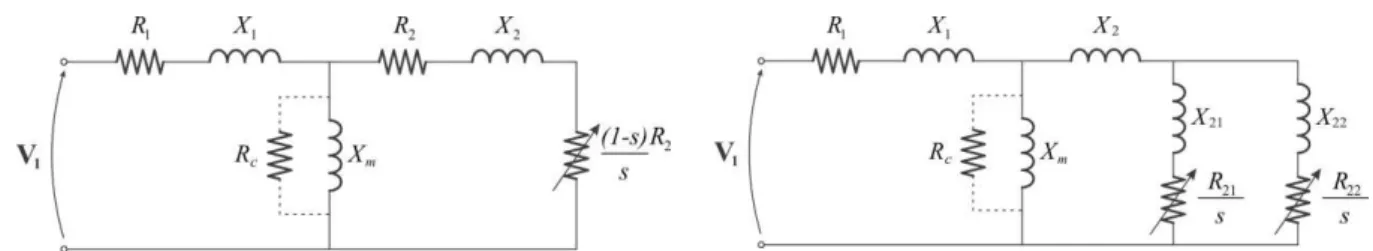
Different models are adopted for each application, as shown in Fig. 1 and Fig. 2. On the single-cage
model, R1 and X1 are the resistance and leakage reactance of the stator, respectively, Rc represents the
core losses, Xm is the magnetizing reactance, R2 and X2 are the resistance and leakage reactance of the
rotor referred to the stator, respectively, s is the per unit slip and V1 is the phase voltage. On the
double-cage model, R21 and X21 correspond to the inner cage resistance and leakage resistance referred
to the stator, while R22 and X22 correspond to the outer cage. The single-cage model without core
losses, depicted on Fig. 1 excluding Rc, usually provides enough precision for torque and current
calculations [3]. For efficiency determination, it is necessary to consider the core losses, added to the
circuit as Rc, as well as friction, winding and stray-load losses, which are considered a posteriori.
Both models with constant parameters are suitable for the operation range between synchronous speed
and maximum torque [4], [5]. In order to properly represent the starting and acceleration conditions, a
double-cage model can be used [4], or the parameters of the single-cage model can be dependent on
the slip [5].
Fig. 1. Single-cage model (SCM) of TIM, may represent core losses (SCM-CL).
Fig. 2. Double-cage model of TIM (DCM), may represent core losses (DCM-CL).
B. Chronological overview
In [6], the parameter values of the single-cage model without core losses (SCM) are identified
through iterative least-squares curve fitting from torque and current measurements at several points
from startup to synchronous speed. Natarajan and Misra [7] pioneered the identification of parameter
values from manufacturer data, using analytical relationships to calculate the single-cage model with
core losses (SCM-CL) in order to build curves of efficiency and power factor. For transient simulation
purposes, [8] employed sensivity analysis to determine the SCM-CL based on catalog data, however
including locked rotor power factor and slip at maximum torque, which are rarely informed by
manufacturers. Rotor parameters R2 and X2 are not considered constant, but functions of slip. Haque
[9] suggests an iterative procedure for the calculation of all SCM-CL and mechanical losses from
catalog data, presenting through the resulting efficiency and power factor curves its superiority over Natarajan and Misra’s method.
To avoid improper convergence, [10] employed genetic algorithms (GA) to find the values of four
parameters of SCM-CL using few experimental data. GA are once more employed in [11] to
are compared among themselves and to Newton’s method, showing that a small deviation on the
initial solution can make the latter to diverge while GA are reliable in this context.
Aiming at field efficiency determination at different intrusion levels, the Oak Ridge National
Laboratory recommended the Nameplate Equivalent Circuit (NEQ) method [12], where the SCM-CL
is derived from the nameplate data by an iterative procedure. A typical deviation of 3.6 % in
efficiency was observed, despite the use of a typical value of rated power factor, given its absence in
NEMA standard nameplates. With a similar objective, [13] uses GA to determine four parameter
values of SCM-CL based on measurements of current and input power at four load conditions. Values
of stray-load losses and ratio of leakage reactances are assumed according to IEEE Std. 112 [1], while
R1 is measured directly.
Genetic algorithms are also used in [14], to determine the parameter values of the double cage
model without core losses (DCM) from catalog data in order to plot torque and current curves, and in
[15], to identify the parameter values of the SCM from current curves for control applications, while
adapting the search space to accelerate convergence.
The identification of SCM parameter values is proposed in [16] by measuring the current waveform
during motor starting and fitting the simulated waveform. In [2], all parameter values of both SCM
and DCM are identified from nameplate data through restricted nonlinear optimization taking into
consideration the effects of saturation.
In [17], the identification of parameter values of the equivalent circuit is analyzed theoretically,
evidencing the existence of a maximum number of parameters that can be univocally determined from
voltage, current and speed measurements. Starting from the equation of per-phase equivalent
impedance as a function of circuit parameters, supply frequency and slip, the concept of model
invariants is introduced as the minimum number of constants that can be achieved by rearranging the
equation. If the number of circuit parameters is greater than the number of model invariants, the
parameter values cannot be determined univocally and additional equations are needed. However, if
the number of parameters is equal to the number of invariants, all parameter values can be determined
as a unique solution. Table I summarizes the numbers of circuit parameters and model invariants for
each of the four models presented previously, evidencing that the equality occurs only in the
SCM-CL. The values of the model invariants can be determined by solving the equations of the real and
imaginary parts of the equivalent impedance at a number of measurement points equal to half the
number of invariants, although additional points are useful to filter deviations.
TABLE I.NUMBER OF CIRCUIT PARAMETERS AND MODEL INVARIANTS BY MODEL [18].
Model Circuit parameters Model invariants
SCM: Single cage 5 4
SCM-CL: Single cage with core losses 6 6
DCM: Double cage 8 6
DCM-CL: Double cage with core losses 9 8
Brazilian Microwave and Optoelectronics Society-SBMO received 15 Sep 2016; for review 16 Sep 2016; accepted 28 Dec 2016
carried out on [18]. Many of the methods described employ the drive systems to perform tests or
impose special excitations during the system startup.
The fsolve function of Matlab is used in [4] to identify parameter values of the SCM and the DCM
based on few catalog data to build torque curves. The same function is used in [5], which aims at
efficiency and torque calculations with the SCM-CL.
In the context of efficiency estimation with SCM-CL, [19] identifies all parameter values from catalog data with analytical expressions. The performances of Newton’s method, Particle Swarm Optimization (PSO) and Simulated Annealing (SA) are compared in [20] by determining four
parameters from low-intrusion field measurements. An iterative linear least-squares method is
employed in [21] to search all parameters based on efficiency and power factor values at four load
levels. A hybrid search method is proposed in [22] to determine four parameter values from current,
power factor and speed measurements. The complete model is calculated in [3] through an iterative
procedure, assuming a typical distribution of losses at rated condition, and through an analytical and
direct method in [23] to obtain torque, current and efficiency curves, which is applied to an extensive
number of motors.
III. ESTIMATION OF PARAMETER VALUES FROM CATALOG DATA
The following data are usually provided by TIM manufacturers on catalogs: rated power Pr; line
voltage Vl; full-load current Ifl; starting current Ist/Ifl; starting torque Tst/Tfl; breakdown torque Tm/Tfl;
efficiency at three load levels (100%), (75%),(50%); power factor at three load levels cos(100%),
cos(75%), cos(50%); rated frequency f; full-load speed N; standard and category. On the nameplate
attached to the machine, only rated power, voltage, frequency, full-load and starting current, full-load
efficiency, power factor and speed are informed.
Some of methods cited in the previous section allow the determination of equivalent circuit
parameter values from catalog data. Others, although originally conceived for field application, can be
converted for this application by employing catalog data as a substitute for measured data. The main
methods are described as follows.
A. Natarajan-Misra’s (NM) Method
In [7], efficiency and power factor are calculated with the SCM-CL, which parameter values are
determined from catalog data. An approximate expression for losses is given by (1), where Po is the
mechanical output power, I1 is the line current and Pconst is the constant loss given by the sum of
friction and windage losses Pfw and core losses Pc. Applying this equation to two load operation points
which data is available on catalog, the system can be algebraically solved for Pconst and (R1+R2). The
core losses are assumed to be equal to one half of the constant losses and the voltage E over the
magnetizing branch is assumed to be approximately equal to V1, thus enabling the calculation of Rc.
2
1 1 2
1
1 3
o const
P I R R P
The magnetizing current Im flowing through Xm (see Fig. 1) is calculated in a similar way by solving
the linear system obtained by applying (2) to two load operation points for Im and (I2sin2), which is
the imaginary part of rotor current referred to the stator I2, while 2 is the rotor impedance angle.
Assuming E approximately equal to V1, Xm can be calculated as E divided by Im.
I2sin2
Im I1sin (2) The real part of the rotor current at full-load is calculated with (3), and its absolute value I2 isdetermined from the real and imaginary parts. Through (4), R2 is determined and subtracted from
(R1+R2) to result in R1. Using the starting and breakdown torques in (5), X2 is calculated and
multiplied to a constant to result in X1.
1
2cos 2 1cos
c
V
I I
R
(3)
2 2 2 3 1 r sP R I s (4)
2 2 2 1 1 st m st mR T T X
T T
(5)
B. Haque’s Method 1
In [9], an iterative method is proposed to identify the parameter values of the SCM-CL for
efficiency and power factor calculation, consisting on the following steps:
1. Line current at 50% of rated load is calculated from efficiency and power factor data, while
initial values are assumed for E, Pfw and I2.
2. R2 results from (6), R1 and Pfw are the solution of the linear system formed by applying (7) to
two load operation points. Rc is calculated from E and Pc equal to half of Pconst, X1 and X2 are
calculated with (8) and fixed ratio X1/X2. Xm is inferred from the reactive power balance.
3. The values of E, I2 and Pfw are updated.
4. Steps 2 and 3 are repeated until convergence.
2 2 2 3 1 r fwP P s
R
I s
(6)
2 2
1 1 2 2
1
3I R 3I R Pconst Po 1
(7)
12 2
21 2 1 2
3 1 fl
st r
T V R
X X s R R
T P
(8)
C. Nolan’s Method
The final objective in [11] is the calculation of torque and current curves from motor starting to
synchronous speed. The authors use GA to search all parameter values of the SCM from starting
Brazilian Microwave and Optoelectronics Society-SBMO received 15 Sep 2016; for review 16 Sep 2016; accepted 28 Dec 2016
From the model, it is possible to express the torque at the three aforementioned conditions as
functions of R1, R2 and total leakage reactance, given by the sum of X1 and X2, assuming that the
parameter values are constant in the desired range and that the magnetizing current is negligible at
starting. An objective function given by the sum of the squares of the deviations between the
calculated torques and the reference values is minimized by the GA. The total reactance is then
divided according to fixed ratios between the reactances, and Xm is finally determined through the
reactive power balance.
D. Nameplate Equivalent Circuit Method (NEQ)
A report from the Oak Ridge National Laboratory (ORNL), presented in [12], assesses methods for
field efficiency estimation and divides them in three groups according to the intrusion level. The NEQ
method, based on the SCM-CL, is pointed as the most precise from the low intrusion group with a
typical deviation of 3.6 %.
The stator resistance is measured directly or, for NEMA design B motors, estimated from (9),
where p is the number of poles and the units of Pr and Vl are horse power and volts, respectively.
4 0.52 1.26 21 1.1 10 r l
R p P V (9)
The stray-load losses are estimated from the percentages suggested on IEEE Std. 112 and are then
included in the circuit as a resistance in the rotor branch. Friction and windage losses are assumed as a
fixed percentage of load input power, equal to 1.2 % for four pole design B motors. Based on
full-load slip, complex equivalent phase impedance, X1/X2 ratio and starting current, the remaining
parameters are iteratively calculated, although the details of the employed algorithm are not provided.
The full-load slip calculated from nameplate data is pointed as the major cause of deviation, since it
has a tolerance of 20 % according to NEMA standards.
E. Sabharwal’s Method
The analytical methodology presented in [19] yields values of the six parameters of the SCM-CL
from catalog data for torque, efficiency and power factor calculation. Friction, windage and stray-load
losses are neglected, while the remaining losses are considered either constant or proportional to the
square of output power, as given in (10). The linear system formed by applying it to two load
operation points is solved for a and Pconst, the latter being fully attributed to Rc, further calculated by
assuming E equal to V1.
2
1
1 Po aPo Pconst
(10)
Neglecting the magnetizing component of the starting current, R2 is approximated by (11), which is
derived from the expression of air-gap power. Using the starting torque, X2 results from (12), and X1
2 1 2 2 3 3 st s c st V T R R I
(11)
2 2 2 1 1 st n st n s T TX R
T T
(12)
The magnitude and phase of the rotor current at full-load are given by (13) and (14), respectively.
The balance of reactive current yields Xm, and finally R1 is determined through the balance of total
losses.
2 2 3 1 r sP I R s (13)
2 2 1 2 arccos I R s V I (14)
F. Lu’s Method
A method for field efficiency assessment employing the SCM-CL is suggested in [20], with few
measurements and no need of load decoupling. The stator resistance is measured directly. The
stray-load losses are estimated according to the percentages of rated power indicated in IEEE Std. 112,
while friction and windage losses are assumed as a fixed percentage of rated power, e.g., 1.2 % for NEMA design B four pole motors below 200 hp. The ratio between X1 and X2 is also fixed according to
the motor design.
The remaining circuit parameters are determined by a numeric optimization algorithm which
minimizes the sum of squares of deviations between calculated and measured data. The real and
imaginary parts of the equivalent impedance are calculated from measured voltage and current
phasors at two load levels, yielding four equations. The solution of the resulting nonlinear system is
performed by three methods: Newton’s method, PSO and SA.
G. Sundareswaran’s Method
The parameter values of the SCM-CL are identified in [22] in a field application with low intrusion,
using a hybrid methodology that combines GA and local search. The algorithm consists of two stages.
In the first one, a GA finds a quasi-optimal solution. Next, a local search method (Rosenbrock’s
rotating coordinates method) further refines the previous solution.
The stator resistance is measured directly, while the ratio of leakage reactances is fixed. By
employing measured values of current, power factor and speed, the remaining parameters are
determined by the hybrid algorithm, which minimizes the sum of squares of deviations of current
magnitude and angle.
H. Haque’s Method 2
Brazilian Microwave and Optoelectronics Society-SBMO received 15 Sep 2016; for review 16 Sep 2016; accepted 28 Dec 2016
values on the slip, thus achieving more precise curves in a wide speed range. MATLAB fsolve
function solves a system of equations consisting of input, output and reactive power at full-load,
breakdown and starting torque.
The author points out that the adopted proportion in the distribution of constant losses between the
mechanical and core components has a small influence on the efficiency deviation, provided that the
total value of constant losses is correct.
I. Lee’s Method
All parameters values of the SCM-CL are identified through a Gauss-Seidel algorithm in [3] in
order to obtain torque versus slip curves, based only on nameplate data: rated output power,
efficiency, power factor, current and speed at full-load, and starting current.
A typical value of 14 % of total losses at full-load is attributed to friction and windage, while 12 %
is attributed to core losses. Stray-load losses Psll are estimated according to the percentages of rated
power indicated on IEEE Std. 112 [1]. This enables the calculation of air-gap power Pag through (15),
followed by R1 through (16) at the full-load condition, where Pin is the input power determined
through nameplate efficiency.
1
o fw sll
ag
P P P
P
s
(15)
1 2
1 3
in c ag
P P P
R
I
(16)
The remaining parameters are estimated with an iterative procedure:
1. Initialize all parameters except R1 as zero, E as phase voltage and I2 as I1cos
2. Calculate R2 with (17);
3. Calculate X1 and X2 with (18) and X1/X2 standard ratios, and Xm from reactive power balance;
4. Calculate Rc from Pc and the current value of E;
5. Compare current parameter values with the previous ones.
a. Stop if convergence is achieved;
b. Update E and I2 and return to step 2.
2 4 2
2
2
4
2 ag
ag
E E P X
R s
P
(17)
12
21 2 2 1 2
st V
X X R R
I
(18)
J. Guimarães’ Method
An analytical non-iterative method is presented in [23] for the estimation of parameter values of the
SCM-CL from catalog or nameplate data. The rotor parameters are considered variable with slip, as
indicated in (19) and (20), where R20 and X20 are the rotor resistance and reactance at starting
2 20exp r 1
R s R g s (19)
2 20exp x 1
X s X g s (20)
Neglecting the stray-load losses, the sum of stator Joule losses and constant losses can be expressed
for any load operation point at steady-state with (21). A linear regression consisting of this expression
at three load conditions usually provided on catalog yields the values of R1 and Pconst. The same is
performed for R2 with (22), by assuming that the rotor Joule losses differ from the stator losses by a
constant amount. For both equations, the slip at partial loads is estimated by (23). Alternative
expressions provide the resistance values from nameplate data only.
2 1 1
1 1
3
1 const o
R I P P
s
(21)
2 2 1
3
1 j r
s
R I K P
s
(22)
0,5 1 1 4 1 o
rated rated r P
s s s
P
(23)
The values of X20, gr and gx are calculated from torque relations, while X1 is determined in order to
match to the starting current. The active power balance yields Rc, accounting for all constant losses,
and Xm is calculated by assuming that the no load current is equal to the reactive part of full-load
current.
After applying the method to a great number of motors, the authors present regressions of the per
unit parameter values versus rated output power.
IV. COMPARISON OF ANALYTICAL METHODS
Among the methods described on the previous section, six stand out for their simplicity, requiring
no numerical optimization routines: Natarajan-Misra’s [7], Haque’s [9], NEQ [12] (for R1 and Pfw
only); Sabharwal’s [19], Lee’s [3] and Guimarães’ [23]. These methods also have in common the
objective of efficiency estimation. The results of these methods can also serve as initial solutions for
more advanced methods, e.g., for the initialization of Newton’s method or for the definition of the
search space of a GA. In this section, the six methods are applied to a set of real motors in order to
compare their performances.
A. Assessment Methodology
The methods are assessed according to two criteria: robustness and precision. The first one
corresponds to the absence of absurd results within numerous executions, such as negative values for
resistances or power. A robust method will not require frequent interventions from the user in order to
overcome eventual divergence, which is suitable for numerous successive executions. Each method
was tested for robustness by the application to 200 low voltage motors with rated power in the range
Brazilian Microwave and Optoelectronics Society-SBMO received 15 Sep 2016; for review 16 Sep 2016; accepted 28 Dec 2016
resulting per unit values of the parameters, having the rated output power and the line voltage as base
values, it was observed if the values formed a well definite value and if there were negative parameter
values.
The second criterion, related to precision, consists on observing the closeness of the resulting values
to reference values. In order to avoid errors due to imprecision in catalog information, these data of
five motors, with rated power ranging from 7.5 to 75 kW, were simulated using circuit parameters
obtained from standard tests, thus reflecting exactly the model. The motors are presented on Table II.
The deviation between the resulting parameters and its reference values is calculated and compared.
TABLE II.DATA FROM THE SIMULATED MOTORS
Motor 1 2 3 4 5
Rated power (kW) 7.5 18.5 37 55 75
Poles 4 2 2 4 6
Voltage (V) 480 380 380 480 440
Current (A) 11.61 35.08 70.35 82.14 128.40
Speed (rpm) 1761.1 3537.1 3559.8 1775.9 1185.2
(100) (%) 90.8 91.5 92.9 93.8 94.6
(75) (%) 91.2 91.4 92.4 93.9 94.8
(50) (%) 90.3 89.9 90.6 92.9 94.4
cos (100) 0.86 0.88 0.86 0.86 0.81
cos (75) 0.81 0.84 0.84 0.83 0.78
cos (50) 0.72 0.77 0.77 0.77 0.70
Tm/Tfl 2.52 2.55 2.23 2.13 1.89
R1 () 0.9101 0.1747 0.0595 0.0701 0.0425
X1 () 1.9006 0.5089 0.3083 0.3443 0.2362
R2 () 0.5450 0.1137 0.0362 0.0464 0.0254
X2 () 2.7950 0.7484 0.4534 0.5063 0.3473
Rc () 1459.0 436.1 193.2 366.5 276.1
Xm () 58.80 17.97 9.23 10.11 4.97
Pfw (W) 35.53 239.30 603.40 460.66 471.46
Psll (W) 51.81 195.81 246.98 418.27 206.55
Pconst (W) 171.35 530.62 1258.40 1007.80 1060.50
B. Results
Fig. 3 to Fig. 7 present the per unit values of circuit parameters resulting from Haque’s method,
taking each motors rated output power and line voltage as base values. The resulting values follow a
well-defined pattern with respect to rated power, the same as observed in other methods with few
exceptions and different maximum and minimum values. The resulting maximum and minimum per
unit values of each parameter for each method are presented on Table III, as well as the count of
0 0,01 0,02 0,03 0,04 0,05 0,06
0 100 200 300 400 500 600
p .u . Pr (hp) R1 R2
Fig. 3. Per unit values of R1 and R2 resulting from Haque’s method.
0 0,005 0,01 0,015 0,02 0,025 0,03
0 100 200 300 400 500 600
p
.u
.
Pr (hp)
X1
Fig. 4. Per unit values of X1 resulting from Haque’s
method. 0 20 40 60 80 100 120 140 160
0 100 200 300 400 500 600
p
.u
.
Pr (hp)
Rc
Fig. 5. Per unit values of Rc resulting from Haque’s method. 0 0,5 1 1,5 2 2,5 3
0 100 200 300 400 500 600
p
.u
.
Pr (hp)
Xm
Fig. 6. Per unit values of Xm resulting from Haque’s method. 0 0,02 0,04 0,06 0,08 0,1 0,12 0,14 0,16 0,18
0 100 200 300 400 500 600
p
.u
.
Pr (hp)
Pconst
Fig. 7. Per unit values of Pconst resulting from Haque’s method.
TABLE III.RESULTING PER UNIT VALUES OF PARAMETERS FROM EACH METHOD
Method Parameters (p.u.)
R1 X1 R2 X2 Rc Xm Pfw
NM Minimum -2.3228 0.0029 0.0032 0.0042 -42.62 0.48 -0.0235
Maximum 0.0485 0.0445 0.0445 0.0654 192.28 17.53 3.0479
Divergences 1 4 - 4 1 - 2
Haque Minimum 0.0065 0.0000 0.0015 0.0000 10.10 0.49 0.0133
Maximum 0.0554 0.0281 0.0210 0.0414 144.19 2.41 0.1697
Divergences - 1 - 1 - - -
NEQ Minimum 0.0219 - - - 0.0124
Maximum 0.2427 - - - 0.0171
Divergences - - - -
Sabharwahl Minimum 0.0062 0.1870 0.0152 0.2750 4.31 0.30 -
Maximum 0.0429 203.6488 22.8037 299.4836 70.20 1.33 -
Divergences - 112 1 138 - 57 -
Lee Minimum 0.0041 0.0286 0.0013 0.0421 14.73 -88.65 0.0049
Maximum 0.0485 0.0613 0.0157 0.0902 223.79 340.69 0.0600
Divergences - - - 108 -
Guimarães Minimum 0.0074 -0.0561 0.0031 0.1102 6.32 0.48 -
Maximum 0.0645 0.0242 0.0416 0.3068 79.17 2.21 -
Brazilian Microwave and Optoelectronics Society-SBMO received 15 Sep 2016; for review 16 Sep 2016; accepted 28 Dec 2016
As can be observed from the highlighted cells in Table III, most of the methods presented at least
one divergence, i.e., one absurd result such as a negative, complex or abnormally high value. From
the methods that yield all circuit parameters, Haque’s method presented the best performance, since it
only resulted in one occurrence of null leakage reactance. The methods of Sabharwahl, Lee and
Guimarães have presented many problems in calculations of reactances, presenting either negative or
absurdly high values. The NEQ resulted in R1 values notoriously greater than other results, although
this is not yet sufficient to disqualify it.
Fig. 8 to Fig. 14 present the results of the precision test, including the parameter Pconst, since the
precision of total constant losses is more important than of its components [5]. The percent deviation
between obtained and reference values is presented for each of the five motors and six methods.
Fig. 8. Percent deviation of R1 resulting from each
method.
Fig. 9. Percent deviation of X1 resulting from each
method.
Fig. 10. Percent deviation of R2 resulting from each
method.
Fig. 11. Percent deviation of X2 resulting from each
method.
Fig. 12. Percent deviation of Rc resulting from each method.
Fig. 14. Percent deviation of Pconst resulting from each method.
Fig. 8 shows that the analytic estimation of R1 from the NEQ method was not appropriate for these
motors, while NM, Haque’s, Sabharwal’s and Guimarães method had a good performance. In
Sabharwal’s method, the high deviation of R2 caused similar deviations on X1 and X2, as shown in
Fig. 9 to Fig. 11. The other methods presented better results for these parameters, except for the
estimation of R2 in Haque’s and Lee’s methods. Fig. 12 shows small deviations in the values of Rc
resulting from NM and Haque’s method, although greater deviations of Pconst are observed in Fig. 14,
meaning that an accurate estimate of Rc does not necessarily imply in a good estimate of constant
losses, as would be preferred instead. Fig. 13 displays the failure of Lee’s method to provide stable
results of Xm, since from five runs, four returned deviations below -100 %, i.e., negative values, and
one returned a deviation of more than 10000 %. Despite employing fixed typical proportions of losses, Lee’s method had the best performance of the calculation of constant losses, as well as NM and Guimarães’ methods.
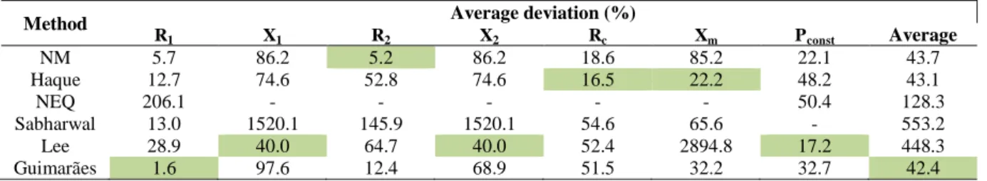
Table IV summarizes the results of this test, indicating for each parameter the average percent
deviation for the five motors analyzed, as well as the average deviation of all parameters for each
method. The highlighted cells refer to the smallest mean deviations obtained at each parameter.
TABLE IV.SUMMARY OF RESULTS FROM THE PRECISION TEST.
Method Average deviation (%)
R1 X1 R2 X2 Rc Xm Pconst Average
NM 5.7 86.2 5.2 86.2 18.6 85.2 22.1 43.7
Haque 12.7 74.6 52.8 74.6 16.5 22.2 48.2 43.1
NEQ 206.1 - - - 50.4 128.3
Sabharwal 13.0 1520.1 145.9 1520.1 54.6 65.6 - 553.2
Lee 28.9 40.0 64.7 40.0 52.4 2894.8 17.2 448.3
Guimarães 1.6 97.6 12.4 68.9 51.5 32.2 32.7 42.4
The smallest global deviation was achieved through Guimarães’ method, responsible also for the
smallest average deviation of R1. Very small deviations were also obtained for R2, Rc and Pconst with
NM, Haque’s and Lee’s methods, respectively. As previously mentioned, Sabharwal’s method has
presented a poor performance in the determination of X1, R2 and X2. The same occurred with Lee’s
method and NEQ for Xm and R1, respectively.
C. Combination of methods
Brazilian Microwave and Optoelectronics Society-SBMO received 15 Sep 2016; for review 16 Sep 2016; accepted 28 Dec 2016
overall deviation and to prevent robustness problems. The proposed method consists on the following:
1. Calculate R1 as in Guimarães’ method [23];
2. Calculate Pc and Pfw as in Lee’s method [3];
3. Calculate R2 as in NM method [7];
4. Calculate X1, X2, Rc and Xmwith Haque’s iterative procedure [9], removing the calculation of
R1, Pconst and R2 and substituting (8) for (18);
The resulting parameter average deviations are presented on Table V. The robustness test with 200
motors returned no divergences.
TABLE V.RESULTS OF THE COMBINED METHOD.
Method Average deviation (%)
R1 X1 R2 X2 Rc Xm Pconst Average
Combined 1.6 41.8 5.2 41.8 51.3 4.7 17.2 23.4
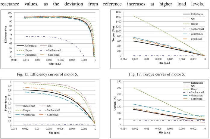
In order to illustrate the influence of deviations in parameter values, curves of efficiency, power
factor, torque and current versus slip were simulated with the resulting values in the speed range from
full-load to synchronous speed. The curves obtained for motor 5 are presented in Fig. 15 through
Fig. 18, which also indicate a reference curve. Sabharwal’s method has presented no closeness at all
with reference curves. The efficiency curves show a good concordance between all remaining methods and the reference curve. The other curves show the predominance of Guimarães’ and the combined method as the most accurate curves. Fig.16 illustrates the effect of inaccurate leakage
reactance values, as the deviation from reference increases at higher load levels.
Fig. 15. Efficiency curves of motor 5.
Fig. 16. Power factor curves of motor 5.
Fig. 17. Torque curves of motor 5.
V. CONCLUSIONS
From the literature review, it was observed that different circuits are used to model the operation of
the three-phase induction motor according to the desired application. For calculations on the normal
operating range, i.e., from maximum torque to no-load condition, the single cage model provides
enough accuracy. For efficiency calculations, the core losses must be considered and are usually
represented by the resistance Rc. If calculations including the starting condition are desired, the single
cage model with constant parameters may not provide enough precision, and a double cage or variable
parameters are considered to improve accuracy.
The alternative methods for parameter value calculation rely basically on analytical calculation, iterative calculations or numerical optimization methods such as Newton’s, genetic algorithms, particle swarm optimization or simulated annealing. The calculations may use manufacturer data,
simple field measurements or detailed laboratory test data.
One advantage of analytical methods is their simplicity and speed, since they do not require the use
of complex or slow algorithms. On the other hand, a lack of robustness was observed in the test
results. From the six tested methods, five presented at least one divergence during the robustness test
with a catalog of 200 motors. The remaining method only provides values for two parameters. The
lack of robustness occurs at different parameters for each method: X1 and X2 diverged frequently in
Sabharwal’s, NM and Haque’s method, Xmin Lee’s method and X1in Guimarães’ method. According
to this test, the most robust methods were Haque’s and NM method.
From the precision test, it was observed that the analytical expression of R1 used in the NEQ has
resulted in large deviations, suggesting that it may be suitable only for a specific group of motors.
While estimating the same parameter value, Guimarães’ method has presented an outstanding
performance, with an average deviation of only 1.6 % from the reference value. Similarly, NM
method has resulted in very small deviations for R1 and R2, despite the simplicity of the method.
Haque’s method resulted in a moderate deviation of Xm. None of the methods, however, had a similar
performance in the calculation of leakage reactance. The estimation of constant losses by typical
percentages of total losses employed in Lee’s method has resulted in small deviations. Still, these
fixed percentages may not be suitable for other motors with different characteristics. Thus, it may be
safer to estimate the constant losses as in NM method, once it takes into account the motors efficiency
vs. load characteristic.
By combining the strong points of each method in terms of robustness and precision, a new method
was proposed and evaluated. Improvements were observed in the precision of the identified parameter
values and resulting curves, as well as in the robustness of the new method, since it had no
malfunctions within 200 runs with different motors. Further tests must be performed with motors of
other manufacturers and characteristics in order to evaluate its performance.
Brazilian Microwave and Optoelectronics Society-SBMO received 15 Sep 2016; for review 16 Sep 2016; accepted 28 Dec 2016
precise match between the circuit parameters and the catalog data. Data provided by manufacturers is
often imprecise, since they refer to a whole group of motors, each with random variations in their
individual characteristics. Tolerances and truncation in the provided values may also add errors to the
calculations.
ACKNOWLEDGMENT
This work was supported by CNPq and an agreement among the GRUCAD/EEL/CTC/UFSC,
ENGIE Brasil SA and IFSC regulated by ANEEL (PD-0403-0034/2013).
REFERENCES
[1] IEEE Standard 112, "IEEE standard procedure for polyphase induction motors and generators," IEEE Nov. 2004, pp. 1-87.
[2] D. Lindenmeyer, H.W. Dommel, A. Moshref, P. Kundur, “An induction motor parameter estimation method,” in International Journal of Electrical Power & Energy Systems, Vol. 23, no. 4, pp 251-262, May 2001.
[3] K. Lee, S. Frank, P. K. Sen, L. G. Polese, M. Alahmad and C. Waters, "Estimation of induction motor equivalent circuit parameters from nameplate data," North American Power Symposium (NAPS), 2012, Champaign, IL, 2012, pp. 1-6. [4] J. Pedra and F. Corcoles, "Estimation of induction motor double-cage model parameters from manufacturer data," in
IEEE Transactions on Energy Conversion, vol. 19, no. 2, pp. 310-317, June 2004.
[5] M. H. Haque, "Determination of NEMA Design Induction Motor Parameters From Manufacturer Data," in IEEE Transactions on Energy Conversion, vol. 23, no. 4, pp. 997-1004, Dec. 2008.
[6] A. Bellini, A. De Carli, M. La Cava, “Parameter identification for induction motor simulation,” in Automatica, vol. 12, no. 4, pp. 383-386, July 1976.
[7] R. Natarajan, V.K. Misra, “Parameter estimation of induction motors using a spreadsheet program on a personal computer,” in Electric Power Systems Research, vol. 16, no. 2, pp 157-164, 1989.
[8] S. Ansuj, F. Shokooh and R. Schinzinger, "Parameter estimation for induction machines based on sensitivity analysis," in IEEE Transactions on Industry Applications, vol. 25, no. 6, pp. 1035-1040, Nov/Dec 1989.
[9] M. H. Haque, “Estimation of three-phase induction motor parameters,” in Electric Power Systems Research, vol. 26, no.3, pp 187-193, 1993.
[10] R. R. Bishop and G. G. Richards, "Identifying induction machine parameters using a genetic optimization algorithm," Southeastcon '90. Proceedings., IEEE, New Orleans, LA, 1990, pp. 476-479 vol.2.
[11] R. Nolan, P. Pillay and T. Haque, "Application of genetic algorithms to motor parameter determination," Industry Applications Society Annual Meeting, 1994., Conference Record of the 1994 IEEE, Denver, CO, 1994, pp. 47-54 vol.1. [12] Kueck, J. D., et al. "Assessment of methods for estimating motor efficiency and load under field conditions." ORNL
(1996).
[13] P. Pillay, V. Levin, P. Otaduy and J. Kueck, "In-situ induction motor efficiency determination using the genetic algorithm," in IEEE Transactions on Energy Conversion, vol. 13, no. 4, pp. 326-333, Dec 1998.
[14] P. Nangsue, P. Pillay and S. E. Conry, "Evolutionary algorithms for induction motor parameter determination," in IEEE Transactions on Energy Conversion, vol. 14, no. 3, pp. 447-453, Sep 1999.
[15] B. Abdelhadi, A. Benoudjit and N. Nait-Said, "Application of genetic algorithm with a novel adaptive scheme for the identification of induction machine parameters," in IEEE Transactions on Energy Conversion, vol. 20, no. 2, pp. 284-291, June 2005. doi: 10.1109/TEC.2004.841508
[16] K. S. Huang, W. Kent, Q. H. Wu and D. R. Turner, "Parameter identification of an induction machine using genetic algorithms," Computer Aided Control System Design, 1999. Proceedings of the 1999 IEEE International Symposium on, Kohala Coast, HI, 1999, pp. 510-515. doi: 10.1109/CACSD.1999.808700
[17] F. Corcoles, J. Pedra, M. Salichs and L. Sainz, "Analysis of the induction machine parameter identification," in IEEE Transactions on Energy Conversion, vol. 17, no. 2, pp. 183-190, Jun 2002. doi: 10.1109/TEC.2002.1009466
[18] H. A. Toliyat, E. Levi and M. Raina, "A review of RFO induction motor parameter estimation techniques," in IEEE Transactions on Energy Conversion, vol. 18, no. 2, pp. 271-283, June 2003. doi: 10.1109/TEC.2003.811719
[19] S. C. Sabharwal, "Methodology for Estimating Performance Characteristics of Three Phase Induction Motor Operating Direct-on-Line or with Six Pulse Inverter," Power Electronics, Drives and Energy Systems, 2006. PEDES '06. International Conference on, New Delhi, 2006, pp. 1-4. doi: 10.1109/PEDES.2006.344343
[20] B. Lu, W. Qiao, T. G. Habetler and R. G. Harley, "Solving Induction Motor Equivalent Circuit using Numerical Methods for an In-Service and Nonintrusive Motor Efficiency Estimation Method," Power Electronics and Motion Control Conference, 2006. IPEMC 2006. CES/IEEE 5th International, Shanghai, 2006, pp. 1-6.
[21] G. Wang and S. W. Park, "Improved Estimation of Induction Motor Circuit Parameters with Published Motor Performance Data," 2014 Sixth Annual IEEE Green Technologies Conference, Corpus Christi, TX, 2014, pp. 25-28. [22] K. Sundareswaran, H. N. Shyam, S. Palani and J. James, "Induction motor Parameter Estimation using Hybrid Genetic
Algorithm," 2008 IEEE Region 10 and the Third international Conference on Industrial and Information Systems, Kharagpur, 2008, pp. 1-6.
[24] F. Corcoles, J. Pedra, M. Salichs and L. Sainz, "Analysis of the induction machine parameter identification," in IEEE Transactions on Energy Conversion, vol. 17, no. 2, pp. 183-190, Jun 2002.