Reursive-Searh Method for Ferromagneti
Ising Systems: Combination with a
Finite-Size Saling Approah
P. C. da Silva,U. L. Fulo
, F. D. Nobre, L. R.da Silva,and L. S.Luena
Departamento deFsiaTeoriaeExperimental
UniversidadeFederaldoRioGrandedoNorte
CampusUniversitario,CaixaPostal1641, 59072-970,Natal,RN,Brazil
Reeivedon19Otober,2001;Revisedversionreeivedon2February,2002
A methodfor obtainingritial properties ofphysial systemsispresented. Basedonareursive
relation involving a physial parameterof the system, it drivesthe system spontaneously to the
ritialpoint,providinganeÆientwaytoestimateritialproperties. Themethodisillustratedfor
several ferromagneti Isingsystemsonwell-knownBravais latties. Anite-sizesalingapproah
isperformed,byapplyingthemethodonlattiesofdierentsizes. TheeÆienyofthemethodis
onrmedbyevaluatingritialtemperatures, aswellasritial exponents,thatturn uptobe in
goodagreementwiththose availableintheliterature,witharelativelysmallomputationaleort.
I Introdution
Although statistial mehanis represents one of the
mostsuessfulphysial theoriesnowadays,onlyafew
simple theoretial models have been solved exatly
withinsuhaframework. Theevaluationofthermal
av-erages, thatare,in priniple,to beperformedoverthe
whole phasespae,beomesahardtaskin mostofthe
ases. As a onsequene, many approximation
meth-ods have been proposed in order to deal with
ompli-ated systems,haraterizedby many-interating
on-stituents. Duetothereentimprovementsinomputer
tehnology,theomputersimulations[1,2,3,4℄beame
nowadays one of the most important tools for
study-ing physial systems. Among many dierent typesof
omputer simulations, one may single out the Monte
Carlo (MC) simulations, that are probably the most
ommonly employedofallnumerialsimulations. The
MC method onsists in performing theusual averages
of statistial mehanisoverarestrited partofphase
spae, i.e., only those ongurations whih ontribute
signiantly to the thermal averages are onsidered;
suh a proedure redues a lot of omputing time, in
suh a way that one may study large { but nite {
physial systems. In a standardMC simulation, eah
dynamial variable (whih may be dened on sites of
regular latties)is visitedeither at random orin
well-dened sequenes,to beafterwardsupdatedaording
toertaindynamialrules;dependingonthesizeofthe
sistem, a MC simulation may require a large
ompu-tational eort. The main drawbak of any numerial
simulationis thatone isrestritedto workwith
nite-sizesystems,andsometimes,thenite-sizeeetsmay
disguise important physial results. A typial ase is
whenoneisworkingwithsystemsat ritiality, where
inordertoobtainreliableresults,oneneedsto
extrap-olatethe data obtained fornite sizes to the
innite-size limit (the so-alled thermodynami limit). The
most ommonly used extrapolation tehnique for
sys-temsexhibiting ritialbehavioristhe nite-size
sal-ing (FSS) approah [1, 2℄. Through the FSS method
oneis ableto extrat ritial properties of aphysial
system, e.g., ritial exponents, from nite-size data;
however,agoodestimateofritialpropertiesrequires
apreisedetermination oftheritialpoint. Although
someFSS methods are able to produe ritial
expo-nents, aswellasthe loationof theritial point, the
appliationofsuhaproedure beomesmuhsimpler
ifoneknowsaprioritheloationoftheritialpoint.
Animportantstepinthetheoryofritial
phenom-enaourredthroughtheoneptofself-organized
riti-ality[5℄,aordingtowhihertaindynamialsystems
evolvespontaneouslytowardstheritialstate,i.e.,the
ritialstateisanattratorofthedynamis. Reently,
theoneptofself-organizedritialityhasbeenapplied
tothe determinationof ritialproperties in polymers
[6℄,perolation[7℄,andmagnetisystems[8,9,10℄. The
methodusesanalgorithmbasedonareursiverelation,
X
n+1 =X
n (Y
n Y
); (1)
involvingtwodimensionlessvariables (X
n ;Y
n
),
ated withparametersof agiven physialsystem. The
variables (X
n ;Y
n
) hange at eah iteration step n, in
suhawaythat afterasuÆientnumberofsteps, X
n
willonvergetoastationaryvalueX
,ompatiblewith
thestationaryvalueY
Y(X
),assumedbyY
n . The
desiredstationarystate(X
;Y
)maybepreviously
se-letedbyanappropriatehoieofthequantityY
;the
rateofonvergenetothestationarystateisontrolled
by theparameter. As an example, fora
ferrromag-neti system, suh quantities may be related to the
temperature and magnetization [8, 9℄ (or to the
tem-perature and inverse of magneti suseptibility [10℄),
respetively;insteadof ontrollingthe temperatureT,
onemayreah ritiality by taking themagnetization
m!0(ortheinverseofsuseptibility1=!0),whih
is equivalent to approahing the ritial temperature,
T ! T
. It is important to mention that the idea of
keepingaphysialparameterofthesystem,assoiated
with the ritial state, lose to asmall positivevalue
(pushing the system automatially to the viinity of
theritialpoint),hasbeenguessedby Sornetteetal.
[11℄, although it wasnot operationally worked out in
termsofareursiverelation.
In the present work we illustrate the algorithm
based on reursive relation (1) by applying it to the
ferromagnetiIsingmodel,denedonsomewell-known
Bravaislatties,namely,thesquare,triangular,
honey-ombandubilatties. Ineahase,thereursive
ap-proahisappliedforseveralnite sizes,andaFSS
ap-proahisperformed. Inspiteofasmallomputational
eort,theritial temperaturesand ritialexponents
obtainedareingoodagreementwiththoseavailablein
theliterature. Inthe nextsetionwedesribethe
nu-merialproedure. Insetion3wepresentanddisuss
ourresults.
II The Numerial Proedure
Let usonsider thenearest-neighbor interation
ferro-magneti Ising model, dened through the
Hamilto-nian,
H= J X
hiji S
i S
j
; (2)
with J >0, and S
i
=1 . Themodel will be
stud-ied on some well-known Bravais latties, namely, the
square,triangular,honeyomb,andubiones. Ineah
ase,severallinearsizesLwill beonsidered;thetotal
number of spins is N = L 2
, for the two-dimensional
latties,andN =L 3
,fortheubilattie.
Forthepresentproblem,theparameterXofEq. (1)
willberelatedtothetemperature,X K=J=(k
B T).
The reursive method is arried out through several
steps,asdesribedbelow[9,10℄.
(a)Onepreviouslydenes(whihontrolstherate
ofonvergene)andY
(whihdenes thedesired
sta-tionarystatetobeaessed).
(b) At the rst iteration, one hooses the initial
value K
0
. This will dene the rangeof parametersto
beinvestigated[(K
n ;Y
n
)willvaryfrom (K
0 ;Y
0 )upto
(K
;Y
)℄.
() Apartiular initial onguration isassigned to
thespinvariablesandthesystemislettoevolve
dynam-ially aording to a given MC presription. Herein,
wehaveusedasinglespin-ip updating,followingthe
Glauberdynamis[12℄, aordingtowhih,
S
i
(t+1)=
1; if z
i (t)p
i (t)
1; if z
i (t)>p
i (t)
when S
i
(t)= 1; (3a)
and
S
i
(t+1)=
1; if z
i
(t)1 p
i (t)
1; if z
i
(t)>1 p
i (t)
when S
i
(t)=1: (3b)
d
Intheequationsabove,z
i
(t)isauniformrandom
num-berin theinterval[0;1℄andp
i
(t)istheprobability
p
i
(t)=f1+exp[ 2h
i (t)℄g
1
; (4a)
where
h
i
(t)=K X
S
j
(t); (4b)
istheloaleldatingonsitei,attimet,andforthe
rstiteration,KK
0
=J=(k
B T
0 ).
(d) After equilibration is attained (t
0
MC steps)
onemayalulatethermodynamiaverages(assoiated
withthepartiularhoieofK
0 )overt
1
MCsteps. To
N
s
samples,i.e.,N
s
distintsequenesofrandom
num-bers. TheaveragevalueY
0
isomputed, andfromEq.
(1) oneobtainsK
1 .
(e) Steps () and (d) are performed for parameter
K
1
,andsoon,insuhawaythatonegets,iteratively,
(K
0 ;Y
0 )!(K
1 ;Y
1 )!(K
2 ;Y
2 ) .
(f)TheproessonvergeswhenY
n andK
n
present
smallosillationsaroundthevaluesY
[denedinstep
(a)℄andK
(thedesiredstationaryvalueofthe
param-eterK),respetively.
(g)Afterthestationaryregimeisattained,onemay
onsider anumbern ofosillationsaround(K
;Y
),
in order to getastatistisforthestationary
tempera-tureT
.
ItisimportanttomentionthatEq. (1)hastwo
pa-rameterstobeadjustedapriori,namely,andY
,in
order to get aproperonvergene ofthe reursive
ap-proah. Theparametermustbesettoasmallvalue;
for an appropriatehoie of Y
, wefound an optimal
value for , below whih K
does not hange within
the error bars: = 10 2
. Thehoie of Y
is
some-what moresubtle; it must behosen aordingto the
desiredstationary state. IfonehoosesY astheorder
parameter of the system, for ahieving a onvergene
towardsritiality, Y
should be set to asmall value
(typially, Y
= 10 2
), whereas for a onvergene to
a low-temperature state, Y
must be set lose to its
maximumvalue. In eah problem afew attempts are
requiredin ordertondtheappropriateY
, insuha
wayastoprovideonvergenetothedesiredstationary
state.
Inthe models investigated herein, one mayhoose
in Eq. (1), Y
n
m
n
[8, 9℄as thedimensionless
mag-netizationperspin(m=N 1
P
i hS
i
i,wherehistands
for athermodynami average). However, for physial
systems exhibiting strong nite-size eets, e.g.,
dis-ordered magnets, the magnetization may present
pro-nounedtailslosetotheritialtemperature,andsuh
a hoie may lead to a large error in the loation of
the ritialtemperature. Foraseslike that,onemay
hooseY
n
astheinverseofaquantitywhihdivergesat
the ritial temperature [10℄; an appropriate quantity
maybethemagnetisuseptibility,
= 1 Nk B T ( h( X i S i ) 2 i h X i S i i 2 ) : (5)
In the present work we estimated the stationary
tem-peratures T
by using Eq. (1) with X
n K n = J=(k B T n
) and Y
n
1=(J
n
)asthe dimensionless
pa-rameterassoiatedwiththemagnetisuseptibility. In
thenextsetionwepresentanddisussourresults.
III Results and Disussion
Fortheresultsthatfollow,wehavesimulatedthemodel
dened through Eq. (2) on two-dimensional latties
(square, triangular, and honeyomb latties) of linear
dimensionsL=20,40,50,and60,andonubilatties
oflinearsizesL=10,12,14,and16. Ateahiteration
n,oursimulationsalwaysstartedwithaompletely
or-deredonguration(allspinsup)andanumberofruns,
orrespondingtoatimet
0 =
1
2
N MC steps,were
dis-ardedbeforealulatingaverages. Afterthat,wehave
omputed thermodynami averagesovert
1
= N MC
steps. All simulations were repeated over N
s = 200
samples,i.e., dierentsequenesofrandomnumbers.
0
100
200
300
400
500
600
n
0.98
1
1.02
1.04
1.06
1.08
1.1
T
L
/T
C
1/(J
χ
∗
L
)=0.050
1/(J
χ
∗
L
)=0.052
1/(J
χ
∗
L
)=0.054
1/(J
χ
∗
L
)=0.056
1/(J
χ
∗
L
)=0.058
Figure1. Evolutionofthetemperature[inunitsofthe
or-responding exat ritial temperature (see Table 1)℄ with
theiterationstepn,fordierenthoiesof
L
,forthe
ferro-magnetiIsingmodelonasquarelattieoflineardimension
L=20. Amongthehoiesinvestigated,theoptimalhoie
orrespondsto 1=(J
L
)=0:054,leading tothe stationary
temperatureT
L =T
=1:04880:0022.
First ofall, in orderto ndthestationary
temper-atureT
L
,assoiatedwitheahlinearsize Lof agiven
lattie,itisimportanttodeterminewithagood
au-raythestationary parameterY
L
=1=(J
L
). InFig.
1wepresenttheevolutionofthetemperaturewiththe
iterationstepn,fordierenthoiesof
L
,forasquare
lattieof linear size L =20; the same isdone for the
magnetisuseptibilityin Fig. 2. FromFigs. 1and2,
onesees learly that there is an optimal value of
L .
Forhoies abovethe optimal value, Eq. (1) will not
onverge to the stationary values, in suh a way that
thetemperaturewilldiverge[e.g.,seetheurveforthe
hoie 1=(J
L
) =0:050 in Fig. 1℄, whereasthe
mag-neti suseptibility will godown after anite number
of iteration steps [e.g., see the urves for the hoies
1=(J
0
50
100 150 200 250 300 350 400 450 500
n
0
5
10
15
20
25
J
χ
L
(a)
0
1000
2000
3000
n
0
5
10
15
20
25
J
χ
L
(b)
0
2000
4000
6000
8000
10000
n
0
5
10
15
20
25
J
χ
L
(c)
Figure2. Evolution ofthedimensionlessmagneti
susep-tibilitywiththeiterationstepn,forsomeofthehoiesof
L
ofFig. 1,fortheferromagnetiIsingmodelonasquare
lattie of linear dimensionL =20. (a)1=(J
L
) = 0:050;
(b) 1=(J
L
) = 0:052; () 1=(J
L
) = 0:054. Among
thehoiesinvestigated, theoptimalhoieorrespondsto
1=(J
)=0:054.
and 1=(J
L
) =0:052 (Fig. 2(b))℄. For hoies below
the optimalvalue, Eq. (1) will onvergeto stationary
valuesthatarenotthoseassoiatedwithritiality;
in-deed, one nds a onvergene to temperature values
belowtheritial temperature [e.g.,see theurvesfor
the hoies 1=(J
L
) = 0:056 and 1=(J
L
)= 0:058 in
Fig. 1℄,whereasthesuseptiblitywillonvergetovalues
that arelowerthantheoneatritiality. Theoptimal
valueof
L
should bethehighesthoieforwhihEq.
(1) onverges to the orresponding stationary values.
For the ases onsidered in Figs. 1 and 2, our
los-est estimate to the optimalvalue is 1=(J
L
) =0:054,
whih leads to a stable onvergene up to iteration
step n = 10 4
, as exhibited in Fig. 2(). Suh a
hoie is assoiated with the stationary temperature
k
B T
L
=J=2:3800:005,representingadisrepanyof
about5%withrespettothewell-knownsquare-lattie
exatritialtemperature(k
B T
=J =2:269185:::).
0
100
200
300
400
500
600
n
0.98
1
1.02
1.04
1.06
T
L
/T
C
L=20
L=40
L=50
L=60
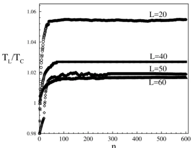
Figure3.Evolutionofthetemperature[inunitsofthe
or-responding exat ritial temperature (see Table 1)℄ with
the iteration step n, for the ferromagneti Ising model
on a honeyomb lattie of dierent linear sizes L. Eah
urve is produed by using the optimal hoie for
L .
The orresponding optimal hoies of
L
, and the
assoi-ated stationary temperatures are: 1=(J
L
) = 0:050 and
kBT
L
=J =1:6020:003 (L=20); 1=(J
L
)=0:015 and
k
B T
L
=J =1:5630:004 (L=40); 1=(J
L
)=0:011 and
k
B T
L
=J =1:5470:008 (L=50); 1=(J
L
)=0:008 and
k
B T
L
=J =1:5430:008 (L=60).
By arrying suh a proedure for dierent linear
sizesofthelattiesonsideredherein,onemaynd
sta-tionarytemperaturesforeahlattiesize. InFig. 3we
exhibittheevolutionofthetemperatureT
L
withthe
it-erationstepnforseveralsizesof ahoneyomblattie;
eahurveofFig. 3isproduedwithitsorresponding
optimal hoie
L
. Onesees that the stationary
tem-peratureapproahestheexatritialtemperaturefor
inreasinglattiesizes. Therefore,onemayextrapolate
the nite-sizestationary temperatures T
L
to the limit
L!1,inordertondthestationarytemperaturesin
thethermodynami limit,T
. Theresultsobtainedin
Fig. 3,forthehoneyomb lattie,areextrapolated
extrap-olated stationary temperatures arepresentedin Table
1forthelattiesonsidered herein. Onesees thattwo
of our extrapolations (honeyomb and ubi latties)
agree,withintheerrorbars,withthevaluesavailablein
the literature,whereasfortheother twoases(square
and triangular latties), we nd a small disrepany
(lessthan1%)withrespettothewell-knownexat
val-ues. Consideringthe modestlattiesizes investigated,
theauray ofthetemperaturesestimatedin Table1
showthepotentialofthereursiveapproahpresented
herein.
Table 1
Square Triangular Honeyomb Cubi
Lattie Lattie Lattie Lattie
k
B T
=J 2:2510:006 3:6050:007 1:5180:006 4:5090:016
k
B T
=J 2:269185::: 3:640956::: 1:518651::: 4:5115250:000003
jT
T
j=T
0.0054 0.0080 { {
Table1: Thedimensionlessstationarytemperatures(k
B T
=J),obtainedbyanextrapolationofseveral
nite-size estimates(k
B T
L
=J)to the limitL !1, for the ferromagnetiIsing model ondierentBravaislatties, are
ompared withtheritialtemperatures(k
B T
=J)availableintheliterature. Forthetwo-dimensionallattiesthe
ritial temperaturesk
B T
=J areknownexatly[13℄, whereasfortheubi lattie,wehaveusedthe estimatesof
Ref. [14℄. Forthehoneyombandubilatties,ourextrapolatedstationary temperaturesagree,within theerror
bars,withtheritialtemperaturesintheliterature;forthesquareandtriangularlatties,ourestimates,inluding
the errorbars, are slightlysmaller thanthe valuesof the literature. Ineah ase, therelativedisrepany of T
(takingintoaounttheerror-barrange)withrespettotheritialtemperature(jT
T
j=T
)isgiven(uptofour
deimaldigits).
0
0.01
0.02
0.03
0.04
0.05
1/L
1.49
1.51
1.53
1.55
1.57
1.59
1.61
k
B
T
*
L
/J
Figure4. Extrapolationofthenite-sizestationary
temper-aturesT
L
,alulatedthroughthereursive-searhmethod,
to the L!1limit, forthe ferromagneti Isingmodelon
ahoneyomblattie. Theextrapolatedstationary
temper-atureisk
B T
=J=1:5180:006.
Let us now onsider the alulation of ritial
ex-ponents through the present method; there are two
straightfowardwaysto arry outsuh aomputation,
as wementionbelow.
(i)Foragivensystemsize,onemayevaluatethe
op-timalvaluefor
L
andonsequentlytheorresponding
stationary temperature T
L
, asdesribedabove. Then,
onemayomputetheritialexponentassoiatedwith
agiventhermodynamipropertybyinvestigatinghow
suhathermodynami propertybehaveswhenone
ap-proahesthestationarytemperatureT
L
. Byrepeating
suh a proedure for dierent system sizes, one may
omputeritialexponentsfordierentsizesandarry
out an extrapolation to the limit L ! 1. This
ap-proah has been applied suessfully for pure [9℄ and
site-diluted [10℄ ferromagneti Ising models, showing
that the reursive method dened by Eq. (1)
ap-proahesritialitythroughtheorretthermodynami
path.
(ii) By knowing the optimal valuefor
L
, one
de-liberatily hooses a
L
above suh an optimal value.
Obviously, there will be no onvergene of the
reur-sionrelationin Eq. (1), andifone startstheiteration
from a suÆiently low temperature, the desired
tem-peraturerange{inludingtheritialregion{maybe
ompletely explored. In this ase, the reursive
rela-tion of Eq. (1) is used in marginal way, determining
thesequene oftemperaturesat whih the
suseptibil-ity will be omputed. By repeating suh aproedure
for dierent lattie sizes, one may obtain the ritial
exponents, as well asthe stationary temperatures, in
thethermodynami limit,byimplementingastandard
FSSapproah[1,2℄.
Inthepresentwork weshallonsiderproedure (i)
fortheloationoftheritialpoint,i.e.,foromputing
stationary temperatures, and proedure (ii) for
om-puting both stationary temperatures and ritial
ex-ponents. In Figs. 5 and 6 we exhibit the
magneti-zationandmagnetisuseptibilityurves,respetively,
obtainedby sheme (ii), for several linear sizes of the
square-lattie model (similar plots hold for the other
latties). Onemaynowusethestandardsaling
Table 2
Square Triangular Honeyomb Cubi
Lattie Lattie Lattie Lattie
k
B T
=J 2:270:01 3:640:02 1:520:01 4:510:02
0:1260:003 0:1240:002 0:1270:003 0:300:03
1:730:04 1:750:02 1:730:03 1:220:02
1:020:02 1:00:02 1:020:04 0:620:01
Table 2: The dimensionless stationary temperatures (k
B T
=J), aswell as the ritial exponents, , and
, asobtainedby aFSS approah, forthe ferromagnetiIsing model ondierent Bravaislatties. All estimated
stationary temperatures agree, within the error bars, with the orresponding ritial temperatures available in
theliterature(seeTable1). Thesamehappens forourritial-exponentestimates,that shouldbeomparedwith
=1=8,=7=4,and =1,whihholdforalltwo-dimensionallatties,duetouniversality[13℄,and =0:3265(3),
=1:2353(11),and=0:6294(5),fortheubilattie[14℄.
m
L
(T)=L =
~ m[L
1=
(T T
)=T
℄;
L
(T)=L =
~ [L
1=
(T T
)=T
℄; (6)
in order to obtain, from our nite-size data, the
sta-tionary temperature T
, as well as the ritial
expo-nents,,and inthethermodynamilimit. InFigs.
7and 8weexhibit thedata olapseof the
magnetiza-tionand suseptibilityurvesshown in Figs. 5and 6,
respetively, forthe square-lattiemodel (similardata
olapsesapplyfortheotherlatties). Theresultsofour
FSSsare exhibitedin Table2,and omparedwiththe
well-knownvaluesavailableintheliterature. Allthe
es-timatedstationarytemperaturesandritialexponents
agree,withintheerrorbars,withthevaluesavailablein
theliterature. Intwoases(squareandtriangular
lat-ties), the stationary temperatures estimated through
asimpleextrapolationto the limitL! 1(f. Table
1), and thoseobtainedby meansof theFSS approah
(f. Table 2), present a small disrepany (inluding
therespetiveerror-barranges). Webelieve thatsuh
disrepaniesareonsequenesofthesmalllattiesizes
investigated.
To onlude, we have investigated the
ferromag-netiIsingmodeldenedonseveralwell-knownBravais
latties, by ombining a reursive method that drives
the system spontaneously towards ritiality, with a
standardFSS approah. Thereursivemethod allows
for the detetion of the ritial temperatures
sponta-neously, through a onvergene towards axed point
of a reursion relation involving a pair of
dimension-lessvariables(X;Y),onstrutedinsuhawaythatX
isassoiatedwiththetemperature,whereasY maybe
related,inpriniple,toanyphysialparameter
display-ing anontrivialbehaviorat ritiality. Inspite ofthe
small omputational eort involved, the eetiveness
ofthemethodhasbeenonrmedbytheevaluationof
ritialtemperaturesandritialexponentsthatarein
good agreementwith those available in theliterature.
0.7
0.8
0.9
1
1.1
1.2
T/T
C
0
0.1
0.2
0.3
0.4
0.5
0.6
0.7
0.8
0.9
1
m
L
L=20
L=40
L=50
L=60
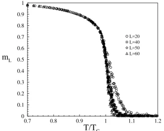
Figure 5. The magnetization per spin plots, versus the
saled temperature, for the ferromagneti Ising model on
squarelattiesofdierentlinearsizes. Thetemperatureis
saledinunitsofthewell-knownexatritialtemperature
ofthemodel(seeTable 1).
0.7
0.8
0.9
1
1.1
1.2
1.3
1.4
T/T
C
0
20
40
60
80
100
120
140
J
χ
L
L=20
L=40
L=50
L=60
Figure6. Plotsofthedimensionlessmagnetisuseptibility
(JL),versusthesaledtemperature(samesaleasinFig.
5), for the ferromagneti Isingmodelonsquare lattiesof
−6
−5
−4
−3
−2
−1
0
1
2
3
4
5
6
[(T−T
*
)/T
*
]L
1/
ν
0
0.2
0.4
0.6
0.8
1
1.2
1.4
1.6
m
L
L
β/ν
L=20
L=40
L=50
L=60
Figure 7. Data olapse of the nite-size magnetization
urvesforthe ferromagnetiIsingmodelonsquarelatties
ofdierentlinearsizes.
−6
−5
−4
−3
−2
−1
0
1
2
3
4
5
6
[(T−T
*
)/T
*
]L
1/
ν
0
0.05
0.1
0.15
(J
χ
L
)L
−
γ/ν
L=20
L=40
L=50
L=60
Figure 8. Data olapse of the nite-sizemagneti
susep-tibilityurvesfor theferromagneti Isingmodelonsquare
lattiesofdierentlinearsizes.
well-known valuesindiatesthat thereursivemethod
yields a onvergene towards ritiality following the
orret thermodynami path. Certainly, the auray
ofpresentresultsmaybesigniantlyimprovedby
us-ing larger lattie sizes. However, we have illustrated
that the power of the method { whih has already
proven its eÆieny in nding ritial properties for
branhedpolymers[6℄, perolation[7℄, pure [8,9℄and
site-diluted[10℄ Ising ferromagnets{ may be
substan-tiallyenhanedifitis ombinedwithaFSSapproah.
Aknowledgments
The partial nanial supports from CNPq, CAPES,
Pronex/MCT,and
ANP/CTPETRO/CENPES/Petrobras (Brazilian
agenies)areaknowledged.
Referenes
[1℄ D.P.LandauandK.Binder,AGuidetoMonteCarlo
Simulationsin StatistialPhysis(Cambridge
Univer-sityPress,Cambridge,2000).
[2℄ M. E. J. Newman and G.T. Barkema, Monte Carlo
Methods in Statistial Physis (Oxford University
Press,Oxford,1999).
[3℄ H.GouldandJ.Tobohnik, AnIntrodution to
Com-puter SimulationMethods, Seond Edition,
(Addison-WesleyPublishingCompany,Reading,Massahusetts,
1996).
[4℄ K. Binder and D. W. Heermann, Monte Carlo
Sim-ulationinStatistial Physis(Springer-Verlag,Berlin,
Heidelberg,1988).
[5℄ P.Bak,C.Tang,andK.Wiesenfeld,Phys.Rev.A38,
364(1988).
[6℄ J.S. AndradeJr., L. S.Luena, A. M. Alenar, and
J.E.Freitas,PhysiaA238,163(1997).
[7℄ A. M. Alenar, J.S. AndradeJr., and L. S. Luena,
Phys.Rev.E56,R2379(1997).
[8℄ U. L. Fulo, L. S. Luena, and G. M. Viswanathan,
PhysiaA264,171(1999).
[9℄ U.L.Fulo,F.D.Nobre,L.R.daSilva,L.S.Luena,
andG.M.Viswanathan,PhysiaA284,223(2000).
[10℄ U. L. Fulo, F. D. Nobre, L. R. da Silva, and L. S.
Luena,PhysiaA297,131(2001).
[11℄ D. Sornette, A. Johansen, and I. Dorni, J. Phys. I
Frane5,325(1995).
[12℄ R.J.Glauber,J.Math.Phys.4,294(1963).
[13℄ R.J.Baxter,ExatlySolvedModelsinStatistial
Me-hanis(AademiPress, London,1982).
[14℄ H.G.Ballesteros, L.A.Fernandez, V.Mart
in-Mayor,
A.Mu~nozSudupe, G.Parisi,and J.J. Ruiz-Lorenzo,